Part II: Stars
Dive into the nature of stars—from our Sun to distant supergiants. Learn how stars are born, how they evolve, and what happens when they die. This part covers the fundamental properties that define stellar characteristics and the cosmic life cycles that shape our universe.
📚 Download Chapter PDFs
Download the original textbook chapters for offline reading and reference:
Chapter 5: The Sun — Our Closest Star
Why Study the Sun?
The Sun is the only star close enough for us to study in exquisite detail. It sits just 1 AU (about 150 million km) away — a mere 8 light-minutes from Earth. Every other star is at least 250,000 times farther. This proximity makes the Sun our astrophysical laboratory: we can resolve features on its surface, measure its vibrations, and even send spacecraft to sample the solar wind directly.
Understanding the Sun is not just academic curiosity. It is the engine that drives climate, weather, and life on Earth. Solar activity affects satellite communications, power grids, and astronaut safety. And because the Sun is a perfectly ordinary G-type main-sequence star, everything we learn about it applies to billions of similar stars in our galaxy.
The Sun at a Glance:
- • Mass: \(M_\odot = 1.989 \times 10^{30}\) kg
- • Radius: \(R_\odot = 6.96 \times 10^{8}\) m
- • Luminosity: \(L_\odot = 3.828 \times 10^{26}\) W
- • Surface Temperature: 5,778 K
- • Age: ~4.6 billion years
- • Spectral Type: G2V
- • Composition: ~73% H, ~25% He, ~2% metals
- • Core Temperature: ~15.7 million K
Solar Structure: Layers of the Sun
The Sun is not a uniform ball of gas. It has a complex, layered structure, much like an onion. Each layer has distinct physical conditions and plays a different role in transporting energy from the core outward to space.
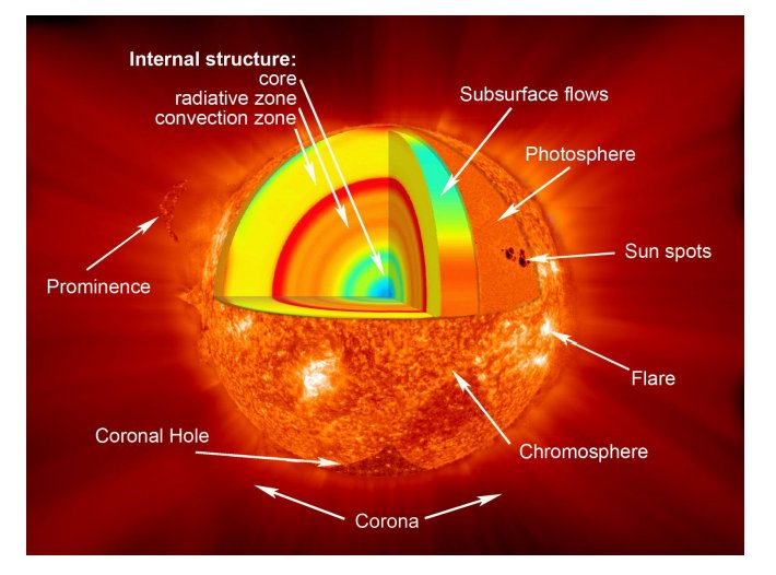
Figure 5.1: The layered structure of the Sun. Energy generated in the core travels outward through the radiative zone, then the convective zone, before escaping from the photosphere.
1. The Core (0 to ~0.25 R)
The innermost region where nuclear fusion takes place. Temperatures reach about 15.7 million K and densities are roughly 150 times that of water. Although the core occupies only about 2% of the Sun's volume, it contains nearly half of its mass and generates 99% of the Sun's energy. Here, hydrogen nuclei are fused into helium through the proton-proton (pp) chain.
2. The Radiative Zone (~0.25 to ~0.7 R)
Energy produced in the core travels outward through this region primarily by radiation — photons are repeatedly absorbed and re-emitted by the dense plasma. The journey through this zone is extraordinarily slow: a single photon may take 100,000 to 170,000 years to random-walk its way from the inner edge to the outer boundary of this zone. The temperature drops from about 7 million K at the base to about 2 million K at the top.
3. The Convective Zone (~0.7 R to surface)
In the outer 30% of the Sun's radius, energy is transported by convection — hot gas rises, cools, and sinks again, much like water boiling in a pot. This is far more efficient than radiation at transporting energy through the relatively cool, opaque gas of this region. The tops of convection cells are visible on the surface as a pattern called granulation.
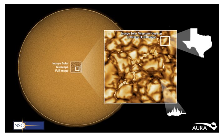
Figure 5.2: Solar granulation. Each granule is the top of a convection cell roughly 1,000 km across. Bright centers show rising hot gas; dark edges show cooler gas sinking back down.
4. The Photosphere (the visible "surface")
This thin layer, only about 500 km thick, is what we see when we look at the Sun. It has a temperature of roughly 5,778 K and is where the Sun's gas becomes transparent enough for photons to escape directly into space. The photosphere is where we observe sunspots — cooler regions (~3,800 K) created by intense magnetic fields that inhibit convection.
5. The Chromosphere
A thin reddish layer above the photosphere, extending about 2,000 km upward. The name comes from the Greek word for "color" because of its pinkish-red hue, visible during total solar eclipses. Surprisingly, the temperature actually increases in this layer, from about 4,400 K at the base to 25,000 K at the top — a phenomenon that puzzled astronomers for decades.
6. The Corona
The Sun's outermost atmosphere, extending millions of kilometers into space. The corona is extraordinarily hot — reaching 1 to 3 million K — yet extremely tenuous (very low density). This extreme heating remains one of the great unsolved problems in solar physics. The corona is visible as a pearly white halo during total solar eclipses.
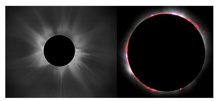
Figure 5.3: The solar corona revealed during a total eclipse. The wispy structures trace magnetic field lines extending millions of kilometers into space.
Nuclear Fusion: The Sun's Power Source
For most of human history, the source of the Sun's energy was a complete mystery. In the 19th century, Lord Kelvin and Hermann von Helmholtz proposed that the Sun was powered by gravitational contraction. But this mechanism could only sustain the Sun's luminosity for about 20 million years — far too short given geological evidence that Earth (and therefore the Sun) is billions of years old.
The answer came from nuclear physics in the 20th century. The Sun is powered by nuclear fusion: the process of combining light atomic nuclei into heavier ones, releasing energy according to Einstein's famous equation \(E = mc^2\). Specifically, four hydrogen nuclei (protons) are fused into one helium-4 nucleus, and the small difference in mass is converted into energy.
The Proton-Proton (pp) Chain:
The dominant energy-generation process in the Sun. The net reaction is:
Four protons become one helium-4 nucleus, two positrons, two electron neutrinos, and gamma-ray photons. The mass of four protons is slightly more than the mass of one helium-4 nucleus. This "missing" mass is converted into energy:
This corresponds to about 0.7% of the original mass. Each reaction releases about 26.7 MeV of energy. The Sun converts roughly 600 million tonnes of hydrogen into helium every second, losing about 4.3 million tonnes of mass as pure energy.
The CNO cycle (carbon-nitrogen-oxygen cycle) is another fusion pathway that uses carbon, nitrogen, and oxygen as catalysts to fuse hydrogen into helium. While the net reaction is the same, the CNO cycle is far more temperature-sensitive and dominates in stars more massive than about 1.3 solar masses. In our Sun, the pp chain produces roughly 99% of the energy.
Mathematical Deep Dive: Solar Energy Output
Optional - Skip if you're just starting out
We can estimate how long the Sun can sustain its current luminosity from nuclear fusion. The solar luminosity is:
Only about 10% of the Sun's hydrogen (the core fraction) is available for fusion, and each kilogram of hydrogen converted releases 0.7% of its rest-mass energy:
The nuclear timescale is then:
Since the Sun is about 4.6 billion years old, it is roughly halfway through its main-sequence lifetime — comforting news for life on Earth!
Solar Activity and the Magnetic Cycle
The Sun is not a static, featureless ball. It is a dynamic, magnetically active star that undergoes an approximately 11-year cycle of activity. During solar maximum, the Sun is covered with sunspots, produces frequent solar flares, and hurls massive clouds of plasma (coronal mass ejections) into space. During solar minimum, the surface is relatively quiet.
Key Features of Solar Activity:
- • Sunspots: Dark patches on the photosphere where intense magnetic fields (~0.3 Tesla) suppress convection, making the region cooler (~3,800 K vs 5,778 K). Sunspots typically appear in pairs with opposite magnetic polarity.
- • Solar Flares: Sudden, intense bursts of radiation caused by the release of magnetic energy through reconnection. Flares can emit across the entire electromagnetic spectrum and accelerate particles to near the speed of light.
- • Coronal Mass Ejections (CMEs): Massive bubbles of magnetized plasma ejected from the corona at speeds of 250 to 3,000 km/s. When directed at Earth, CMEs can cause geomagnetic storms, disrupt satellites, and create stunning auroral displays.
- • Solar Wind: A continuous stream of charged particles (mostly protons and electrons) flowing outward from the corona at 300-800 km/s, filling interplanetary space and creating the heliosphere.
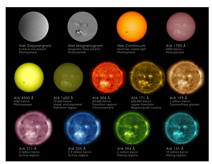
Figure 5.4: The Sun observed at different wavelengths by NASA's Solar Dynamics Observatory (SDO). Each wavelength reveals different layers and temperatures of the solar atmosphere.
The 11-year sunspot cycle is actually half of a 22-year magnetic cycle. During each cycle, the Sun's global magnetic field reverses polarity. The mechanism driving this cycle is the solar dynamo — a complex interaction between the Sun's differential rotation (the equator rotates faster than the poles) and convective motions that amplify and reconfigure the magnetic field.
Key Insight:
The Sun is an average star in nearly every respect — mass, luminosity, temperature, and age. This is actually good news for astrophysics: by studying the Sun in detail, we build a solid foundation for understanding the billions of Sun-like stars in our galaxy, and by extension, for understanding the conditions for life elsewhere in the universe.
For Graduate Students
Explore the full mathematical treatment of stellar structure equations, energy transport mechanisms, and nuclear reaction networks:
Chapter 6: Stellar Characteristics
Classifying the Stars
When you look up at the night sky, every star appears as a simple point of light. But astronomers have discovered that stars come in an extraordinary variety — from tiny, cool red dwarfs barely larger than Jupiter to blazing blue supergiants a million times more luminous than the Sun. How do we make sense of this diversity? The answer lies in classification: organizing stars by their measurable properties to reveal the underlying physics.
Spectral Classification: OBAFGKM
In the early 20th century, astronomers at Harvard Observatory — led by Annie Jump Cannon — classified hundreds of thousands of stellar spectra. They developed a system based on the strength of absorption lines, which turned out to be a sequence of decreasing surface temperature. The modern spectral classification runs: O, B, A, F, G, K, M (remembered by the mnemonic "Oh Be A Fine Girl/Guy, Kiss Me").
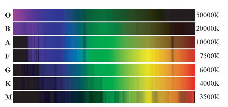
Figure 6.1: Spectra of stars across the spectral sequence. The pattern of absorption lines changes systematically with temperature, reflecting which atoms and ions are present in the stellar atmosphere.
The Spectral Types:
> 30,000 K. Blue. Very hot and luminous. Strong ionized helium lines. Rare — only 1 in 3 million stars. Examples: massive stars in the Orion Nebula.
10,000 - 30,000 K. Blue-white. Neutral helium lines prominent. Example: Rigel, Spica.
7,500 - 10,000 K. White. Very strong hydrogen (Balmer) lines — the strongest of any spectral type. Examples: Sirius, Vega.
6,000 - 7,500 K. Yellow-white. Weakening hydrogen lines; ionized metal lines appear. Example: Procyon, Canopus.
5,200 - 6,000 K. Yellow. Ionized calcium lines strong; many metal lines. Our Sun is a G2V star.
3,700 - 5,200 K. Orange. Neutral metal lines dominate. Examples: Arcturus, Aldebaran.
< 3,700 K. Red. Molecular bands (especially titanium oxide, TiO) appear. The most common type — about 76% of all stars. Example: Betelgeuse, Proxima Centauri.
Each spectral class is further divided into subclasses numbered 0 through 9, with 0 being the hottest within each class. So a B0 star is hotter than a B9, and B9 is close in temperature to an A0 star. The Sun, classified as G2, is slightly hotter than the middle of the G range.
Luminosity Classes
Spectral type tells us a star's surface temperature, but two stars with the same temperature can have vastly different luminosities if they differ in size. A red supergiant and a red dwarf might both be spectral type M, but the supergiant is millions of times more luminous because it is enormously larger.
To capture this distinction, astronomers add a luminosity class to the spectral type. This is determined by subtle differences in spectral line widths — giant stars have narrower absorption lines because their atmospheres are less dense.
Luminosity Classes (Morgan-Keenan system):
- • Ia, Ib: Supergiants (e.g., Betelgeuse, Rigel)
- • II: Bright giants
- • III: Giants (e.g., Arcturus, Aldebaran)
- • IV: Subgiants
- • V: Main-sequence dwarfs (e.g., the Sun = G2V, Sirius = A1V)
The full classification of the Sun is G2V — spectral type G, subclass 2, luminosity class V (main sequence).
The Hertzsprung-Russell Diagram
The most important diagram in all of stellar astrophysics is the Hertzsprung-Russell (HR) diagram, independently developed by Ejnar Hertzsprung and Henry Norris Russell around 1910. It plots stellar luminosity (or absolute magnitude) against surface temperature (or spectral type/color). What could have been a random scatter of points turns out to reveal profound structure.
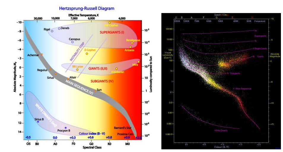
Figure 6.2: The Hertzsprung-Russell diagram. Stars are not randomly distributed — they cluster in distinct regions that correspond to different stages of stellar evolution.
Key Features of the HR Diagram:
- • The Main Sequence: A broad band running diagonally from hot, luminous blue stars (upper left) to cool, dim red stars (lower right). About 90% of all stars lie on the main sequence — these are stars that are fusing hydrogen into helium in their cores, just like the Sun. Position on the main sequence is determined primarily by mass.
- • Red Giant Branch: A region of cool but very luminous stars in the upper right. These are evolved stars that have exhausted the hydrogen in their cores and expanded enormously. Their large surface area compensates for their lower temperature.
- • White Dwarf Region: Hot but very dim stars in the lower left. These are the remnant cores of dead low-mass stars, roughly the size of Earth but with the mass of the Sun. We will explore these in Chapter 8.
- • Supergiants: The most luminous stars, spanning the top of the diagram. These massive stars are rare but spectacularly bright.
Why the Main Sequence Exists:
The main sequence is not just an observational pattern — it reflects fundamental physics. The luminosity and temperature of a hydrogen-fusing star are both determined by a single parameter: its mass. More massive stars have stronger gravity compressing their cores, which drives faster fusion rates, producing higher luminosities and higher surface temperatures. This is why the main sequence is a mass sequence: the most massive stars sit at the top left and the least massive at the bottom right.
The Stefan-Boltzmann Law and Stellar Sizes
How can we determine the radius of a distant star we can never visit? The answer lies in the Stefan-Boltzmann law, which connects a star's luminosity, radius, and surface temperature:
The Stefan-Boltzmann Law:
where \(L\) is luminosity, \(R\) is stellar radius, \(\sigma = 5.67 \times 10^{-8}\,\text{W m}^{-2}\text{K}^{-4}\) is the Stefan-Boltzmann constant, and \(T\) is surface temperature.
If we measure a star's luminosity (from its brightness and distance) and its temperature (from its spectrum or color), we can solve for its radius. This is how we know that red giants are hundreds of times the Sun's size, and white dwarfs are roughly Earth-sized.
The Mass-Luminosity Relation
For main-sequence stars, there is a remarkably tight relationship between mass and luminosity. Observationally, this relation is approximately:
This means a star twice the mass of the Sun is roughly \(2^{3.5} \approx 11\) times more luminous. A star ten times the Sun's mass is roughly \(10^{3.5} \approx 3,200\) times more luminous! This has a profound consequence: massive stars burn through their fuel supply far faster than low-mass stars.
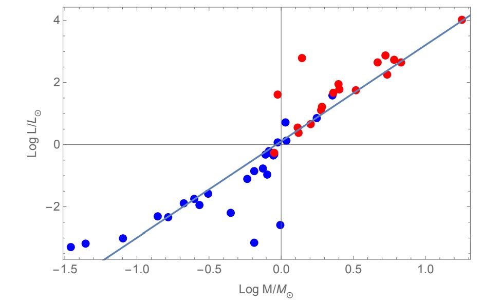
Figure 6.3: The mass-luminosity relation for main-sequence stars. Luminosity increases steeply with mass, roughly as the 3.5 power.
Mathematical Deep Dive: Wien's Law and Stellar Colors
Optional - Skip if you're just starting out
Wien's displacement law tells us the peak wavelength of a star's thermal emission:
where \(b = 2.898 \times 10^{-3}\,\text{m}\cdot\text{K}\) is Wien's displacement constant. For the Sun at 5,778 K:
This falls in the green part of the visible spectrum (though the Sun appears white/yellow because it emits strongly across all visible wavelengths). For a hot O-type star at 40,000 K,\(\lambda_{\text{max}} \approx 72\) nm (ultraviolet), and for a cool M-type star at 3,000 K,\(\lambda_{\text{max}} \approx 966\) nm (near-infrared).
This is why hot stars appear blue and cool stars appear red: their peak emission shifts through the visible spectrum with temperature.
Chapter Summary:
Stars are classified by spectral type (temperature) and luminosity class (size/evolutionary state). The HR diagram organizes this information visually and reveals that the main sequence is a mass sequence. The Stefan-Boltzmann law connects luminosity, radius, and temperature, while the mass-luminosity relation shows that mass is the single most important property determining a main-sequence star's characteristics.
For Graduate Students
Dive deeper into stellar atmospheres, opacity theory, and the physics behind spectral line formation:
Chapter 7: Stellar Evolution
The Life Stories of Stars
Stars are not eternal. They are born, they live, and they die — but on timescales so vast that no human civilization has ever witnessed the full life cycle of a single star. Yet astronomers have pieced together the complete story by observing billions of stars at different stages, much like understanding the human lifespan by photographing a crowd of people at various ages.
The key insight of stellar evolution is deceptively simple: a star's fate is determined almost entirely by one property — its initial mass. Mass determines how hot the core gets, how fast the fuel is consumed, how long the star lives, and what it becomes when it dies. In astrophysics, mass is destiny.
Star Formation: From Gas to Starlight
Stars are born inside giant molecular clouds — enormous, cold, dark regions of interstellar space filled with molecular hydrogen (H₂) and dust. These clouds can be tens to hundreds of light-years across and contain enough material to form thousands of stars. Typical conditions inside a molecular cloud: temperature around 10-20 K, density around 10³ to 10⁶ particles per cm³.
For a cloud (or a region within it) to collapse under its own gravity and form a star, its gravitational energy must exceed its thermal (pressure) energy. This critical condition defines a minimum mass required for collapse, called the Jeans mass.
The Jeans Mass:
The minimum mass a cloud must have for gravity to overcome thermal pressure and initiate collapse:
where \(k_B\) is Boltzmann's constant, \(T\) is the cloud temperature, \(G\) is the gravitational constant, \(m_H\) is the hydrogen mass, and \(\rho\) is the gas density. For typical molecular cloud conditions, the Jeans mass is a few solar masses. Colder or denser regions have lower Jeans masses, enabling the formation of lower-mass stars.
Collapse can be triggered by various events: a passing shock wave from a nearby supernova, compression from spiral arm passage in the galaxy, or collision between clouds. Once collapse begins, the cloud fragments into smaller clumps, each forming an individual star or stellar system.
Stages of Star Formation:
- Cloud Fragmentation: A massive molecular cloud breaks into smaller clumps, each destined to form one or a few stars.
- Protostellar Collapse: Each fragment contracts under gravity. As it shrinks, gravitational energy is converted to heat, and the center becomes a protostar — an opaque, hot core surrounded by an infalling envelope of gas and dust.
- Pre-Main-Sequence: The protostar continues to contract and heat up, radiating mainly in the infrared. A protoplanetary disk often forms around it. The star is visible as a T Tauri star (for low masses) or Herbig Ae/Be star (for intermediate masses).
- Main Sequence Arrival: When the core temperature reaches about 10 million K, hydrogen fusion ignites. The star reaches hydrostatic equilibrium — the outward pressure from fusion exactly balances the inward pull of gravity. It has joined the main sequence.
Life on the Main Sequence
The main sequence is the longest phase of a star's life — the period during which it fuses hydrogen into helium in its core. How long this phase lasts depends critically on two factors: the total fuel supply (proportional to mass) and the rate of fuel consumption (the luminosity).
Main-Sequence Lifetime:
Since the fuel supply scales with mass and the consumption rate scales with luminosity:
Calibrating to the Sun (\(t_{\text{MS},\odot} \approx 10\) billion years):
Main-Sequence Lifetimes by Mass:
- • 60 M☉ (O-type): ~3 million years
- • 10 M☉ (B-type): ~30 million years
- • 3 M☉ (A-type): ~500 million years
- • 1.5 M☉ (F-type): ~3 billion years
- • 1 M☉ (G-type, Sun): ~10 billion years
- • 0.5 M☉ (K-type): ~60 billion years
- • 0.1 M☉ (M-type): ~trillions of years
The smallest red dwarfs will outlive every other type of star — and indeed will still be shining long after the current age of the universe has been dwarfed by their lifespans.
Mathematical Deep Dive: The Kelvin-Helmholtz Timescale
Optional - Skip if you're just starting out
Before nuclear fusion was understood, Lord Kelvin and Hermann von Helmholtz proposed that the Sun was powered by gravitational contraction. The timescale for this process gives us a useful estimate of how long a protostar takes to contract:
For the Sun:
Compare this to the nuclear timescale of ~10 billion years. The Kelvin-Helmholtz timescale is about 300 times shorter — gravitational contraction simply cannot power the Sun for long enough. This was the "age of the Sun" problem that nuclear physics resolved.
However, the KH timescale is relevant for pre-main-sequence evolution: it tells us roughly how long a protostar takes to contract from a cloud fragment to a main-sequence star.
Post-Main-Sequence Evolution
When a star exhausts the hydrogen in its core, it can no longer support itself against gravity through core hydrogen fusion. What happens next depends on the star's mass, but the general pattern is dramatic expansion and transformation.
Evolution of a Sun-like Star (1 M☉):
- Hydrogen Shell Burning: When core H is exhausted, an inert helium core forms. Hydrogen fusion continues in a shell around the core. The core contracts and heats while the outer layers expand and cool.
- Red Giant Branch: The star swells to 50-100 times its original radius, becoming a red giant. Surface temperature drops to ~3,500 K (hence the red color), but luminosity increases enormously because of the huge surface area. The star moves to the upper-right region of the HR diagram.
- Helium Flash: In low-mass stars (below ~2.3 M☉), the helium core becomes so dense that it is supported by electron degeneracy pressure. When the core reaches ~100 million K, helium fusion ignites explosively — the helium flash. This happens in seconds but is absorbed internally; it is not visible from outside.
- Horizontal Branch: After the helium flash, the star settles into a stable phase of core helium fusion (the "triple-alpha" process, fusing helium into carbon) surrounded by hydrogen shell burning. The star is smaller and hotter than on the red giant branch.
- Asymptotic Giant Branch (AGB): When core helium is exhausted, the star again expands to become a giant — now even larger and more luminous. The star has two burning shells (hydrogen and helium) around an inert carbon-oxygen core. AGB stars experience thermal pulses and intense mass loss through stellar winds.
- Planetary Nebula & White Dwarf: The outer layers are gently expelled, forming a beautiful, glowing planetary nebula. The exposed hot core remains as a white dwarf — the subject of Chapter 8.
Mass Determines Fate
The evolution described above applies to stars similar to the Sun. More massive stars follow a different path — they burn through successive nuclear fuels much faster, and their endings are far more dramatic.
Stellar Fates by Initial Mass:
Low Mass (\(M < 0.5\,M_\odot\)):
These red dwarfs burn hydrogen so slowly that they will remain on the main sequence for trillions of years — far longer than the current age of the universe. No low-mass star has ever died of old age. They are fully convective, meaning they can fuse nearly all their hydrogen, eventually becoming helium white dwarfs.
Intermediate Mass (\(0.5 - 8\,M_\odot\)):
Stars like the Sun follow the evolutionary path described above: main sequence, red giant, AGB, planetary nebula, and finally a carbon-oxygen white dwarf. More massive stars in this range evolve faster and produce more massive white dwarfs.
High Mass (\(M > 8\,M_\odot\)):
These massive stars can fuse elements all the way up to iron in their cores. When the iron core reaches a critical mass, it collapses catastrophically, triggering a core-collapse supernova. The remnant is a neutron star or, for the most massive progenitors, a black hole. We explore these dramatic endpoints in Chapter 8.
Key Takeaway:
Stellar evolution is not random — it is governed by well-understood physics. A star's initial mass determines its temperature, luminosity, lifetime, evolutionary path, and ultimate fate. The HR diagram is not just a snapshot but a map of stellar evolution, showing where stars spend different phases of their lives.
For Graduate Students
Study the detailed physics of stellar evolution, including the equations of stellar structure, nucleosynthesis networks, and computational stellar models:
Chapter 8: Stellar Remnants
The Endpoints of Stellar Evolution
When a star has exhausted its nuclear fuel, what remains? The answer depends on the mass of the remnant core, and it leads us to some of the most extreme and fascinating objects in the universe: white dwarfs, neutron stars, and black holes. These stellar remnants push the laws of physics to their limits and reveal phenomena — from quantum degeneracy pressure to the warping of spacetime — that have no parallel in everyday experience.
White Dwarfs: Quantum Stars
White dwarfs are the remnant cores of low- and intermediate-mass stars (initial mass below about 8 M☉). After the star has shed its outer layers as a planetary nebula, the remaining core is an incredibly dense object roughly the size of Earth but with a mass comparable to the Sun. A teaspoon of white dwarf material would weigh about 5 tonnes on Earth.
What supports a white dwarf against gravitational collapse? It is no longer generating energy through nuclear fusion. Instead, it is held up by electron degeneracy pressure — a quantum mechanical effect arising from the Pauli exclusion principle. Electrons, being fermions, resist being compressed into the same quantum state. This creates an outward pressure that is independent of temperature.
White Dwarf Properties:
- • Mass: 0.2 to 1.4 M☉ (typical ~0.6 M☉)
- • Radius: ~6,000-10,000 km (Earth-sized)
- • Density: ~10⁹ kg/m³
- • Surface Temp: 4,000 to 150,000 K (initially very hot)
- • Composition: Carbon-oxygen (most common)
- • Support: Electron degeneracy pressure
A remarkable property of white dwarfs is that more massive ones are actually smaller. Adding mass compresses the electrons further, shrinking the star. This inverse mass-radius relationship has a critical limit:
The Chandrasekhar Limit:
Discovered by Subrahmanyan Chandrasekhar in 1930 (at just 19 years old!), this is the maximum mass that electron degeneracy pressure can support. Above this limit, even electrons moving at nearly the speed of light cannot generate enough pressure. If a white dwarf exceeds the Chandrasekhar mass — for example, by accreting matter from a companion star — it will collapse or explode. This plays a crucial role in Type Ia supernovae.
White dwarfs produce no new energy. They simply cool over billions of years, fading from white-hot through yellow, orange, and red, eventually becoming invisible "black dwarfs." However, the universe is not yet old enough for any white dwarf to have fully cooled — the oldest are still warm enough to detect.
Supernovae: Cosmic Explosions
Supernovae are among the most energetic events in the universe. For a few weeks, a single supernova can outshine an entire galaxy of 100 billion stars. There are two fundamentally different types:
Type Ia Supernovae (Thermonuclear):
These occur in binary star systems where a white dwarf accretes matter from a companion star. When the white dwarf's mass approaches the Chandrasekhar limit (~1.4 M☉), carbon and oxygen fusion ignites throughout the entire star in a runaway thermonuclear explosion. The white dwarf is completely destroyed — no remnant is left behind.
Because all Type Ia supernovae explode at roughly the same mass, they all have roughly the same peak luminosity. This makes them excellent "standard candles" for measuring cosmic distances. Type Ia supernovae were used to discover the accelerating expansion of the universe in 1998, leading to the 2011 Nobel Prize in Physics.
Core-Collapse Supernovae (Type II, Ib, Ic):
These mark the death of massive stars (initial mass above ~8 M☉). After exhausting hydrogen, these stars fuse progressively heavier elements in their cores — helium to carbon, carbon to neon, neon to oxygen, oxygen to silicon, and finally silicon to iron. This creates an "onion-shell" structure with layers of different elements.
Iron is the endpoint because iron fusion does not release energy — it requires energy input. When the iron core grows to about 1.4 M☉ (the Chandrasekhar mass), electron degeneracy pressure can no longer support it. The core collapses in less than a second, falling inward at up to 70,000 km/s (about 25% the speed of light).
The collapse is halted when the core reaches nuclear density (~10¹⁷ kg/m³), creating a "bounce" that sends a powerful shock wave outward through the star. This shock wave, aided by neutrinos carrying 99% of the explosion energy, blows the outer layers of the star into space. The remnant core becomes either a neutron star or a black hole.
Neutron Stars and Pulsars
When a massive star's iron core collapses, protons and electrons are squeezed together to form neutrons (via inverse beta decay: \(p + e^- \rightarrow n + \nu_e\)). The result is a neutron star — an object of astonishing density composed almost entirely of neutrons, supported by neutron degeneracy pressure and nuclear forces.
Neutron Star Properties:
- • Mass: 1.4 to ~2.2 M☉
- • Radius: ~10 km (city-sized!)
- • Density: ~10¹⁷ kg/m³ (nuclear density)
- • Magnetic Field: 10⁸ to 10¹⁵ T
- • Rotation: Milliseconds to seconds per revolution
- • Surface Gravity: ~10¹¹ times Earth's
A sugar-cube-sized piece of neutron star material would weigh about 1 billion tonnes on Earth. The entire mass of the Sun would be compressed into a sphere roughly the diameter of a large city.
Many neutron stars are observed as pulsars — rapidly rotating neutron stars that emit beams of radio waves (and sometimes X-rays and gamma rays) from their magnetic poles. As the star rotates, these beams sweep across the sky like a cosmic lighthouse. If a beam happens to cross Earth, we detect regular pulses of radiation with extraordinary precision.
Pulsars were first discovered in 1967 by Jocelyn Bell Burnell and Antony Hewish. The signals were so regular that they were initially dubbed "LGM-1" (Little Green Men), half-jokingly suggesting an alien origin. The fastest known pulsars (millisecond pulsars) rotate over 700 times per second — their surfaces move at a significant fraction of the speed of light.
Black Holes: Where Gravity Wins
For the most massive stellar cores (above roughly 2-3 M☉ after the supernova explosion), not even neutron degeneracy pressure can halt the collapse. The matter continues to compress without limit, forming a black hole — a region of spacetime where gravity is so extreme that nothing, not even light, can escape.
The Schwarzschild Radius:
The boundary of a black hole — the point of no return — is called the event horizon. For a non-rotating black hole, the radius of the event horizon is given by:
where \(G\) is the gravitational constant, \(M\) is the black hole mass, and \(c\) is the speed of light. For a black hole of one solar mass:
A stellar black hole of 10 solar masses would have an event horizon only about 30 km across — smaller than a city. The entire mass is concentrated at a point of infinite density called the singularity (though most physicists believe a proper theory of quantum gravity will resolve this infinity).
Black holes cannot be observed directly (by definition — they emit no light). Instead, we detect them through their effects on nearby matter. Gas falling toward a black hole forms a swirling accretion disk that heats up to millions of degrees, emitting intense X-rays. In binary systems, we can also infer a black hole's presence from the orbital motion of a visible companion star.
In 2015, the LIGO observatory made the first direct detection of gravitational waves — ripples in spacetime produced by the merger of two black holes about 1.3 billion light-years away. This monumental discovery confirmed a key prediction of Einstein's general relativity and opened an entirely new window on the universe. In 2019, the Event Horizon Telescope collaboration produced the first direct image of a black hole's shadow — the supermassive black hole at the center of galaxy M87.
Mathematical Deep Dive: Escape Velocity and Black Holes
Optional - Skip if you're just starting out
The Schwarzschild radius can be derived from a simple (though not fully rigorous) Newtonian argument. The escape velocity from a mass \(M\) at radius \(r\) is:
Setting \(v_{\text{esc}} = c\) (the speed of light) and solving for \(r\):
Remarkably, this Newtonian derivation gives the same result as Einstein's general relativity (though this is partly coincidental). The physical interpretation in GR is much richer: at\(r = r_s\), time effectively stops for a distant observer, and space itself "flows" inward faster than the speed of light.
Summary: The Three Stellar Remnants
White Dwarf
- • Progenitor: \(M < 8\,M_\odot\)
- • Remnant mass: \(< 1.4\,M_\odot\)
- • Size: Earth
- • Support: electron degeneracy
- • Density: ~10⁹ kg/m³
Neutron Star
- • Progenitor: \(8 - 25\,M_\odot\)
- • Remnant mass: \(1.4 - 2.2\,M_\odot\)
- • Size: ~10 km
- • Support: neutron degeneracy
- • Density: ~10¹⁷ kg/m³
Black Hole
- • Progenitor: \(> 25\,M_\odot\)
- • Remnant mass: \(> 3\,M_\odot\)
- • Size: \(r_s = 2GM/c^2\)
- • Support: none (singularity)
- • Density: infinite at center
The Big Picture:
Stellar remnants are far more than cosmic curiosities. White dwarfs in binary systems produce Type Ia supernovae that serve as cosmic distance markers. Neutron star mergers forge heavy elements like gold, platinum, and uranium through rapid neutron capture (the r-process). Black holes power the most luminous objects in the universe — quasars and active galactic nuclei. And gravitational waves from compact object mergers are opening an entirely new era in astronomy. The deaths of stars are not endings — they are the seeds of new cosmic phenomena.
For Graduate Students
Explore the advanced physics of compact objects, general relativity, and high-energy astrophysics: