Sun-Earth Interactions & Space Weather
1. Solar Structure & Corona
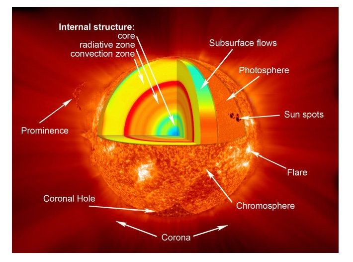
The Sun's internal structure — from the nuclear-burning core through the radiative and convective zones to the photosphere, chromosphere, and corona.
The Sun is a main-sequence G2V star with mass $M_\odot = 1.989 \times 10^{30}$ kg and radius$R_\odot = 6.957 \times 10^{8}$ m. Energy is generated in the core via the pp-chain and CNO cycle, transported radiatively to $\sim 0.7\,R_\odot$, then convectively to the photosphere.
Hydrostatic Equilibrium
Throughout the solar interior, pressure balances gravity:
where $M(r) = 4\pi \int_0^r \rho(r') r'^2 \, dr'$ is the enclosed mass. Combined with the equation of state$P = \frac{\rho k_B T}{\mu m_p}$ (ideal gas), the opacity law, and nuclear energy generation rates, this yields the stellar structure equations.
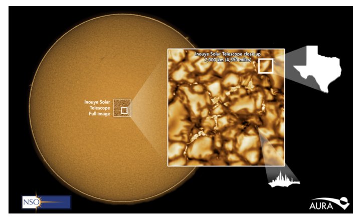
Solar granulation imaged by the Daniel K. Inouye Solar Telescope — convective cells ~1000 km across carry energy to the photosphere.
The Corona
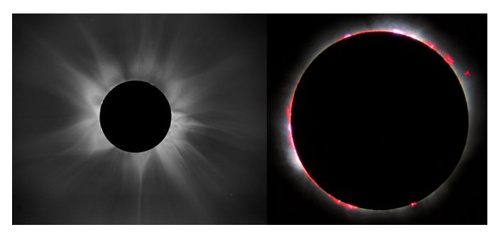
The solar corona revealed during a total eclipse — the white-light K-corona (electron scattering) and red chromospheric prominences.
Above the photosphere ($T \approx 5800$ K), temperature drops through the chromosphere then rises sharply across the transition region to coronal values $T \sim 1$–$3 \times 10^6$ K. This temperature inversion — the coronal heating problem — remains one of solar physics' grand challenges.
Coronal Scale Height
In an isothermal corona, the density falls exponentially with a gravitational scale height:
For $T = 1.5 \times 10^6$ K and mean molecular weight $\mu \approx 0.6$, we get $H \approx 100$ Mm, giving $n(r) = n_0 \exp\left[-\frac{R_\odot}{H}\left(1 - \frac{R_\odot}{r}\right)\right]$.
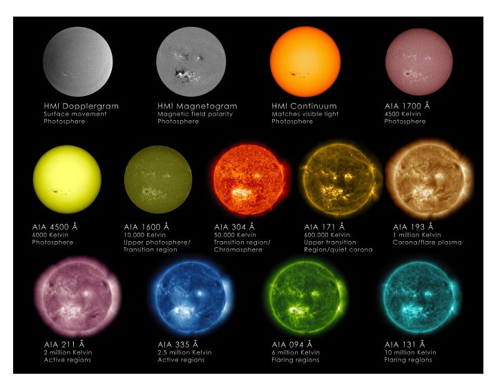
The Sun at multiple wavelengths (SDO/AIA) — each channel probes a different temperature, from the photosphere (HMI, 5800 K) to flaring plasma (AIA 131 Å, 10 MK).
Coronal Heating Mechanisms
The corona requires a heating rate of $\sim 300$ W m$^{-2}$ in active regions. Leading candidates:
- AC heating (wave dissipation): Alfvén waves propagate from the photosphere and dissipate via phase mixing, resonant absorption, or turbulent cascade
- DC heating (nanoflares): Braiding of magnetic field lines by photospheric convection drives small-scale reconnection events (Parker 1988)
2. Solar Dynamo & Magnetic Fields
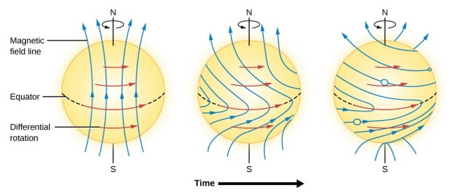
The solar dynamo — differential rotation stretches the poloidal field into a toroidal field (Ω-effect), producing bipolar sunspot pairs that migrate toward the equator.
The Sun's magnetic field is generated by a magnetohydrodynamic (MHD) dynamo operating at the interface between the radiative and convective zones — the tachocline at $\sim 0.7\,R_\odot$.
Magnetic Induction Equation
The evolution of the magnetic field in a conducting fluid is governed by:
The first term represents advection/stretching of field lines by plasma flow; the second is Ohmic diffusion with magnetic diffusivity $\eta = 1/(\mu_0 \sigma)$. The magnetic Reynolds number$R_m = v L / \eta$ determines which dominates. For the Sun, $R_m \sim 10^{10}$, so the field is frozen into the plasma.
The α-Ω Dynamo
The solar dynamo operates via two coupled processes in mean-field electrodynamics ($\mathbf{B} = \overline{\mathbf{B}} + \mathbf{b}'$):
Ω-effect: Differential rotation ($\Omega(r,\theta)$) stretches poloidal field into toroidal field. The angular velocity gradient at the tachocline is key:$\partial B_\phi / \partial t \sim r \sin\theta\, B_r \, \partial\Omega/\partial r$.
α-effect: Helical turbulent convection twists toroidal field back into poloidal field. The mean EMF $\overline{\mathcal{E}} = \alpha \overline{\mathbf{B}} - \beta \nabla \times \overline{\mathbf{B}}$where $\alpha \propto -\frac{\tau}{3}\langle \mathbf{v}' \cdot (\nabla \times \mathbf{v}') \rangle$ encodes the kinetic helicity.
Sunspot Cycle
The $\sim 11$-year Schwabe cycle (22-year magnetic cycle) arises from the dynamo oscillation. Sunspots appear where buoyant magnetic flux tubes ($B \gtrsim 10^5$ G) pierce the photosphere. Hale's law: leading/following spots have opposite polarity in opposite hemispheres, reversing each cycle. Joy's law: bipolar regions are tilted $\sim 5°$–$10°$ toward the equator.
3. Solar Flares & Coronal Mass Ejections
Solar flares and coronal mass ejections (CMEs) are the most energetic phenomena in the solar system, releasing $10^{25}$–$10^{32}$ ergs in minutes to hours via magnetic reconnection.
The CSHKP Model
The standard flare model (Carmichael, Sturrock, Hirayama, Kopp-Pneuman) describes a two-ribbon flare: a rising flux rope drives reconnection in the current sheet below, creating cusp-shaped post-flare loops. The reconnection rate is controlled by the inflow Alfvén Mach number:
Energy release rate: $\dot{W} \approx \frac{B^2}{2\mu_0} v_{\text{in}} L^2$ where $L$ is the current sheet length. For $B = 100$ G, $L = 10^{9}$ cm, $M_A = 0.01$–$0.1$, this gives $\dot{W} \sim 10^{28}$–$10^{29}$ erg/s.
CME Dynamics
CMEs are expelled when the confining magnetic field can no longer contain the rising flux rope. The torus instability criterion: the critical decay index of the overlying field is $n_{\text{crit}} \approx 1.5$:
Once launched, a CME propagates through the heliosphere subject to aerodynamic drag against the solar wind. The drag-based equation of motion (Vršnak et al. 2013):
where $\gamma = c_d A \rho_{\text{sw}} / M_{\text{CME}} \sim 10^{-8}$–$10^{-7}$ km$^{-1}$. Fast CMEs ($v > v_{\text{sw}}$) decelerate; slow CMEs accelerate toward $v_{\text{sw}}$.
Simulation: CME Drag-Based Propagation
PythonModel CME propagation from Sun to 1 AU using the aerodynamic drag equation.
Click Run to execute the Python code
Code will be executed with Python 3 on the server
4. Solar Energetic Particles
Solar energetic particles (SEPs) are ions and electrons accelerated to MeV–GeV energies by solar flares (impulsive events) and CME-driven shocks (gradual events). They pose significant radiation hazards to astronauts and spacecraft.
Diffusive Shock Acceleration (DSA)
At CME-driven shocks, particles undergo first-order Fermi acceleration. Repeated crossings of the shock produce a power-law energy spectrum. For a shock with compression ratio $s = \rho_2/\rho_1$:
For a strong shock ($s = 4$), $\sigma = 4$, corresponding to a differential energy spectrum$dJ/dE \propto E^{-1}$. The acceleration timescale depends on the diffusion coefficient$\kappa$ upstream and downstream of the shock.
Parker Transport Equation
SEP transport in the heliosphere is governed by the Parker transport equation for the pitch-angle-averaged distribution $f(\mathbf{r}, p, t)$:
Terms: convection by solar wind, spatial diffusion (parallel $\kappa_\parallel$ and perpendicular$\kappa_\perp$ to $\mathbf{B}$), adiabatic deceleration, and source $Q$. The parallel mean free path $\lambda_\parallel = 3\kappa_\parallel / v$ ranges from 0.01 to 1 AU depending on particle rigidity and interplanetary turbulence levels.
5. The Solar Wind
The solar wind is a continuous supersonic outflow of plasma from the solar corona, first predicted theoretically by Eugene Parker (1958) and confirmed by Mariner 2 in 1962. It fills the heliosphere and carries the Sun's magnetic field to the outer reaches of the solar system.
Parker's Isothermal Wind Model
For steady, spherically symmetric, isothermal outflow, the momentum equation:
With $P = \rho c_s^2$ (isothermal) and mass continuity $\rho v r^2 = \text{const}$, this yields Parker's equation:
The critical point where $v = c_s$ occurs at the sonic radius:
The unique transonic solution that starts subsonic at the solar surface, passes through $r_c$, and becomes supersonic is the solar wind solution. At 1 AU, the solar wind reaches$v \approx 300$–$800$ km/s with $n \approx 5$ cm$^{-3}$.
Fast and Slow Solar Wind
Two distinct wind regimes exist:
- Slow wind ($\sim 300$–$400$ km/s): originates from streamer belt regions near the heliospheric current sheet; variable, dense ($n \sim 10$ cm$^{-3}$), composition closer to coronal loops
- Fast wind ($\sim 600$–$800$ km/s): emanates from coronal holes (open field regions); steady, tenuous ($n \sim 3$ cm$^{-3}$), photospheric composition, higher proton temperature
Simulation: Parker Solar Wind Solutions
PythonSolve Parker's isothermal wind equation for transonic and breeze solutions.
Click Run to execute the Python code
Code will be executed with Python 3 on the server
6. Interplanetary Magnetic Field
The solar magnetic field is carried outward by the solar wind plasma (frozen-in condition). Because the Sun rotates with angular velocity $\Omega_\odot \approx 2.87 \times 10^{-6}$ rad/s, the field lines are wound into the Parker spiral.
Parker Spiral
In the equatorial plane, assuming radial wind speed $v_r = v_{\text{sw}}$ = const and$v_\phi = 0$ far from the Sun, the steady-state field components are:
The garden-hose angle — the angle between the field and the radial direction — is:
At Earth's orbit ($r = 1$ AU), for $v_{\text{sw}} = 400$ km/s: $\psi \approx 45°$. The IMF magnitude at 1 AU is typically $B \approx 5$–$10$ nT.
Sector Structure
The heliospheric current sheet (HCS) separates regions of opposite magnetic polarity. It is warped due to the tilt of the solar magnetic dipole relative to the rotation axis, creating a "ballerina skirt" pattern. As the Sun rotates, Earth crosses sectors of alternating polarity, producing the two-sector or four-sector IMF pattern observed at 1 AU.
IMF $B_z$ Component
The north-south component of the IMF ($B_z$ in GSM coordinates) is the single most important parameter controlling solar wind–magnetosphere coupling. When $B_z < 0$ (southward), reconnection occurs at the dayside magnetopause, driving geomagnetic activity. The coupling function of Akasofu (1981):
where $\theta_c = \arctan(B_y/B_z)$ is the IMF clock angle and $\ell_0 \approx 7\,R_E$is the effective magnetopause coupling length.
7. The Bow Shock
The supersonic solar wind cannot penetrate Earth's magnetosphere directly. A standing bow shock forms upstream, typically at $\sim 13$–$15\,R_E$along the Sun-Earth line, where the solar wind is decelerated, heated, and deflected around the magnetopause.
Rankine-Hugoniot Jump Conditions
Conservation of mass, momentum, and energy across the shock yields the MHD Rankine-Hugoniot relations. For a perpendicular shock (B normal to shock normal), the density compression ratio:
where $M_f = v_1 / v_f$ is the fast magnetosonic Mach number and $\gamma = 5/3$. For strong shocks ($M_f \gg 1$), $\rho_2/\rho_1 \to (\gamma+1)/(\gamma-1) = 4$. Typical solar wind: $M_f \approx 6$–$8$, giving compression $\sim 3.5$–$3.8$.
Bow Shock Standoff Distance
The subsolar standoff distance can be estimated from pressure balance and gasdynamic theory. The Spreiter et al. (1966) relation:
where $\Delta = R_{bs} - R_{mp}$ is the shock-magnetopause distance and $R_{mp}$is the magnetopause standoff distance. For $M = 8$, $\Delta/R_{mp} \approx 0.28$, so $R_{bs} \approx 1.28\,R_{mp} \approx 13$–$15\,R_E$.
Quasi-Parallel vs Quasi-Perpendicular Shock
The character of the bow shock depends on $\theta_{Bn}$, the angle between the upstream magnetic field and the shock normal:
- Quasi-perpendicular ($\theta_{Bn} > 45°$): clean, sharp transition; specularly reflected ions
- Quasi-parallel ($\theta_{Bn} < 45°$): diffuse, extended transition; upstream backstreaming ions create foreshock turbulence
8. The Magnetosheath
The magnetosheath is the region of shocked solar wind plasma between the bow shock and magnetopause. The plasma here is subsonic, compressed ($n \sim 20$–$40$ cm$^{-3}$), heated ($T \sim 10^6$ K), and turbulent.
Plasma Properties
Across the bow shock, the solar wind is compressed and heated. Post-shock plasma beta:
In the magnetosheath, $\beta \gg 1$ near the bow shock (thermal pressure dominates), decreasing toward the magnetopause where $\beta \sim 1$. Near the subsolar magnetopause, a plasma depletion layer (PDL) forms: magnetic field piles up against the obstacle, squeezing out plasma ($B \uparrow$, $n \downarrow$, $\beta \downarrow$). The PDL is most prominent for northward IMF.
Flow Pattern
Magnetosheath plasma flows around the magnetopause following streamlines governed by the gasdynamic equations. The flow speed increases from zero at the stagnation point (subsolar) to supersonic at the flanks. The velocity field approximately satisfies:
for potential flow around a blunt obstacle. The magnetic field drapes around the magnetopause, creating a characteristic draping pattern that affects reconnection geometry at the magnetopause.
Magnetic Reconnection — Fundamental Physics
Magnetic reconnection is the fundamental plasma process by which magnetic field lines of opposite polarity break and reconnect, converting stored magnetic energy into kinetic energy, thermal energy, and particle acceleration. It is the key mechanism powering solar flares, driving magnetospheric dynamics, and enabling solar wind entry into the magnetosphere.
The Frozen-In Condition and Its Breakdown
In ideal MHD ($R_m \to \infty$), Alfvén's theorem states that magnetic flux is conserved through any surface moving with the plasma — field lines are "frozen in". The electric field is:
Reconnection requires this condition to break down in a localized diffusion regionwhere non-ideal terms become important. The generalized Ohm's law:
The terms on the right represent, respectively: resistive diffusion, the Hall term(decouples ion and electron motion at the ion inertial length $d_i = c/\omega_{pi}$), the electron pressure tensor (off-diagonal terms break frozen-in at the electron scale$d_e = c/\omega_{pe}$), and electron inertia.
Sweet-Parker Model (1957–58)
The simplest steady-state reconnection model assumes a long, thin current sheet of length $L$(system scale) and half-width $\delta$. Inflow at speed $v_{\text{in}}$ carries oppositely directed field lines toward the sheet, where they diffuse through resistive dissipation and reconnect. Plasma is ejected at the Alfvén speed $v_A$ from the sheet ends.
Combining these gives the reconnection rate (inflow Alfvén Mach number):
where $S$ is the Lundquist number. For the magnetopause:$L \sim 10\,R_E$, $v_A \sim 200$ km/s, $\eta/\mu_0 \sim 1$ m$^2$/s, giving $S \sim 10^{13}$ and $M_A \sim 3 \times 10^{-7}$. This is$\sim 10^5$ times slower than observed — the Sweet-Parker problem.
Derivation: Sweet-Parker Reconnection Rate
Consider a rectangular diffusion region of length $2L$ and width $2\delta$:
1. Incompressible mass conservation: $v_{\text{in}} \cdot L = v_{\text{out}} \cdot \delta$
2. Outflow pressure balance (inflow magnetic pressure → outflow kinetic energy):$\frac{B^2}{2\mu_0} = \frac{1}{2}\rho v_{\text{out}}^2$, so $v_{\text{out}} = v_A = B/\sqrt{\mu_0\rho}$
3. Inflow Ohm's law at the center of the sheet: $E_z = v_{\text{in}}B = \eta J_z = \eta B/(\mu_0\delta)$, so $v_{\text{in}} = \eta/(\mu_0\delta)$
4. Eliminate $\delta$: From (1): $\delta = L v_{\text{in}}/v_A$. Substitute into (3):$v_{\text{in}} = \eta v_A / (\mu_0 L v_{\text{in}})$, giving $v_{\text{in}}^2 = \eta v_A/(\mu_0 L)$
Petschek Model (1964)
Petschek proposed that the diffusion region need not span the entire system scale. Instead, it is compact ($\ll L$), and standing slow-mode shocks attached to the X-point extend outward, converting most of the magnetic energy outside the diffusion region:
For $S = 10^{13}$: $M_A \approx 0.013$, yielding $v_{\text{in}} \approx 2.5$ km/s — consistent with observations at the magnetopause ($M_A \sim 0.01$–$0.1$). The reconnection rate depends only logarithmically on $S$, making it nearly independent of resistivity.
Hall Reconnection and the Two-Scale Structure
Modern kinetic simulations reveal that fast reconnection arises from the Hall effect. The diffusion region has a two-scale structure:
- Ion diffusion region ($\sim d_i \approx 100$ km at magnetopause): ions decouple from field lines and follow meandering orbits; characterized by a quadrupolar out-of-plane magnetic field $B_y$ — the Hall magnetic field signature
- Electron diffusion region ($\sim d_e \approx 2$ km): electrons decouple; off-diagonal electron pressure tensor breaks the frozen-in condition; the reconnection electric field is sustained by electron-scale physics
The Hall currents create a characteristic pattern: the in-plane Hall current $\mathbf{J}_H = (n_e e)(\mathbf{v}_i - \mathbf{v}_e)$produces a quadrupolar $B_M$ (guide field component) structure that is a diagnostic signature of ongoing reconnection, detected by spacecraft such as MMS.
Reconnection Rate: The 0.1 Problem
Both kinetic simulations and observations consistently show a reconnection rate:
independent of $S$, system size, or plasma parameters — the so-called "0.1 problem". This universality arises because the Hall effect opens the exhaust angle to $\sim 0.1$ radians, set by the aspect ratio of the ion diffusion region. The reconnection electric field:
Energy Conversion and Partition
The total energy conversion rate in reconnection:
where $L_X$ is the X-line length and $L_Z$ the current sheet extent. Energy is partitioned approximately as:
- ~50% → bulk kinetic energy of exhaust jets ($v_{\text{out}} \sim v_A$)
- ~25% → ion thermal energy (viscous heating in the exhaust)
- ~15% → electron thermal energy (parallel heating along separatrices)
- ~10% → non-thermal particle acceleration (power-law tails)
Asymmetric Reconnection
At the magnetopause, reconnection is asymmetric — the magnetosheath and magnetospheric plasmas have very different densities and field strengths. The Cassak-Shay (2007) scaling for asymmetric reconnection gives:
where subscripts 1 and 2 denote the two sides. The X-point shifts toward the weaker-field (magnetosheath) side, and the exhaust is asymmetric with different speeds on each side.
Guide Field Reconnection
When a significant magnetic field component $B_g$ exists parallel to the X-line (the guide field), the reconnection geometry changes qualitatively. The quadrupolar Hall field is distorted, the separatrices become asymmetric, and electron acceleration occurs preferentially along the guide field direction. The reconnection rate remains $\sim 0.1$ for $B_g \lesssim B_0$ but decreases for very strong guide fields. At the magnetopause, $B_g/B_0 \sim 0.1$–$3$ depending on IMF $B_y$.
Tearing Instability and Plasmoid Formation
Long current sheets are unstable to the tearing mode. The growth rate for a Harris sheet:
For $S > S_c \sim 10^4$, the current sheet fragments into a chain of magnetic islands (plasmoids) connected by secondary X-lines. This plasmoid-mediated reconnectionleads to bursty, intermittent energy release. In the magnetotail, plasmoid formation is observed as flux ropes traveling tailward, detected as bipolar $B_z$ signatures.
Reconnection in Different Contexts
| Context | L (m) | B (T) | S | Observed $M_A$ |
|---|---|---|---|---|
| Solar flares | $10^7$ | $10^{-2}$ | $10^{12}$–$10^{14}$ | 0.001–0.1 |
| Magnetopause | $10^7$ | $5 \times 10^{-8}$ | $10^{12}$–$10^{13}$ | 0.01–0.1 |
| Magnetotail | $10^8$ | $2 \times 10^{-8}$ | $10^{13}$–$10^{14}$ | 0.01–0.2 |
| MRX lab | 0.3 | $5 \times 10^{-2}$ | $10^2$–$10^3$ | 0.1–0.3 |
MMS Mission: Direct Observation of Electron Diffusion Region
NASA's Magnetospheric Multiscale (MMS) mission (launched 2015) achieved the first direct observation of electron-scale reconnection at the magnetopause. With 30 ms resolution and 7.5 km spacecraft separation (comparable to $d_e$), MMS detected:
- Crescent-shaped electron velocity distributions in the diffusion region
- The electron-scale reconnection electric field $E_R \sim 2$ mV/m
- Agyrotropy of the electron pressure tensor breaking frozen-in
- Electron acceleration to $\sim 100$ keV at the X-point and along separatrices
These observations confirmed the Hall reconnection picture with two-scale structure and validated decades of kinetic simulation predictions.
9. Magnetopause Structure
The magnetopause is the boundary separating the shocked solar wind (magnetosheath) from the Earth's magnetosphere. It is a thin current layer ($\sim 800$ km) maintained by the diamagnetic drift of magnetosheath and magnetospheric particles.
Chapman-Ferraro Pressure Balance
At the subsolar point, the magnetopause location is determined by pressure balance between solar wind dynamic pressure and magnetospheric magnetic pressure:
For a dipole field $B_{mp} = B_0(R_E/R_{mp})^3$ (with $B_0 \approx 3.12 \times 10^{-5}$ T), the standoff distance:
For typical solar wind ($n = 5$ cm$^{-3}$, $v = 400$ km/s),$R_{mp} \approx 10\,R_E$. Including the factor $f \approx 2.44$ for the dipole compression by magnetopause currents: $B_{mp} = f B_0 (R_E/R_{mp})^3$.
Shue et al. (1998) Empirical Model
The magnetopause shape is well described by the Shue et al. model using solar wind dynamic pressure $D_p$ (nPa) and IMF $B_z$ (nT):
where the standoff distance and flaring parameter are:
10. Dayside Reconnection
When the IMF has a southward component ($B_z < 0$), magnetic reconnection occurs at the dayside magnetopause, merging interplanetary and geomagnetic field lines. This is the primary mechanism for solar wind energy entry into the magnetosphere (Dungey, 1961).
Sweet-Parker Reconnection
In the simplest steady-state model (Sweet 1958, Parker 1957), reconnection occurs in a thin, elongated current sheet of length $L$ and width $\delta$:
where $S$ is the Lundquist number. For solar/magnetospheric plasmas, $S \sim 10^{12}$–$10^{14}$, giving $M_A \sim 10^{-6}$ — far too slow to explain observed reconnection rates.
Petschek Reconnection
Petschek (1964) showed that standing slow-mode shocks attached to a compact diffusion region can accelerate the outflow, giving:
For $S = 10^{12}$, $M_A \approx 0.014$ — consistent with observed reconnection rates. Modern kinetic simulations show that the Hall effect and electron-scale physics are essential for enabling fast reconnection.
Flux Transfer Events (FTEs)
Dayside reconnection is often intermittent and spatially patchy, producing flux transfer events(Russell & Elphic, 1978) — bundles of reconnected magnetic flux that propagate along the magnetopause. FTEs have a characteristic bipolar $B_N$ signature (normal component) with enhanced $|B|$. Each FTE transfers $\sim 10^6$–$10^7$ Wb of magnetic flux, contributing to the Dungey cycle polar cap flux budget.
Reconnection Rate and Cross-Polar Cap Potential
The dayside reconnection electric field maps along open field lines to the ionosphere, driving the cross-polar cap potential:
where $L_X$ is the reconnection X-line length. Typical values: $\Phi_{PC} \sim 30$–$150$ kV, reaching $\sim 200$+ kV during strong southward IMF.
11. Dungey Cycle & Magnetospheric Convection
The Dungey cycle (1961) describes the global circulation of magnetic flux driven by reconnection: dayside reconnection opens geomagnetic field lines, the solar wind carries them over the poles into the tail, where nightside reconnection closes them, returning flux to the dayside.
Convection Electric Field
The solar wind imposes an electric field on the magnetosphere via the frozen-in condition:
For southward IMF, this gives a dawn-to-dusk electric field $E_y \approx v_{\text{sw}} |B_z|$across the magnetosphere. Plasma drifts sunward with velocity $\mathbf{v}_E = \mathbf{E} \times \mathbf{B}/B^2$.
Ionospheric Convection
The magnetospheric convection maps to a two-cell pattern in the ionosphere: antisunward flow over the polar cap (open field lines) and sunward return flow at lower latitudes (closed field lines). The total potential drop:
where $\epsilon$ is Akasofu's coupling function in watts. Under northward IMF, lobe reconnection creates reverse (sunward) convection cells at high latitudes.
12. The Plasmasphere
The plasmasphere is a torus of cold ($\sim 1$ eV), dense ($\sim 10^2$–$10^4$ cm$^{-3}$) plasma that corotates with the Earth. It extends to $L \approx 4$–$6$ during quiet times and is the dominant cold plasma reservoir in the inner magnetosphere.
Corotation and the Plasmapause
The corotation electric field in the equatorial plane:
where $\Omega_E = 7.27 \times 10^{-5}$ rad/s. The plasmapause forms where the corotation potential equals the convection potential. The Carpenter-Anderson (1992) empirical model:
During storms ($Kp = 7$–$9$), the plasmasphere erodes to $L \approx 2$–$3$. Drainage plumes form on the duskside, connecting to the magnetopause and feeding cold plasma into the reconnection region.
13. The Magnetotail
The magnetotail extends antisunward for $> 200\,R_E$, consisting of two lobes of opposite polarity magnetic field separated by the plasma sheet. The cross-tail current sustains the stretched tail configuration.
Harris Current Sheet
The central plasma sheet can be modeled as a Harris equilibrium (1962), a one-dimensional solution of the Vlasov-Maxwell equations:
where $\delta$ is the half-thickness ($\sim 1$–$5\,R_E$ during quiet times, thinning to $\sim 0.1\,R_E$ before substorm onset) and $B_0 \approx 20$–$30$ nT is the lobe field strength.
Lobe Magnetic Flux
The total magnetic flux in each tail lobe:
where $R_T \approx 20$–$30\,R_E$ is the tail radius and $B_{\text{lobe}} \approx 20$ nT. This gives $\Phi_{\text{lobe}} \approx 0.5$–$0.8$ GWb. Changes in lobe flux drive substorm dynamics.
14. Polar Cusps
The polar cusps are funnel-shaped regions near $\sim 78°$–$80°$magnetic latitude where magnetosheath plasma has direct access to the ionosphere along field lines connected to the magnetopause.
Cusp Geometry and Velocity Filter
Reconnected field lines at the dayside magnetopause are swept poleward by the solar wind. Magnetosheath ions entering along these field lines undergo a velocity filter effect: at the equatorward edge of the cusp, only the fastest ions have time to reach the ionosphere before being convected poleward. Moving poleward through the cusp, progressively slower (lower energy) ions are observed, producing the characteristic energy-latitude dispersion:
The cusp is a diamagnetic cavity — the influx of magnetosheath plasma depresses the local magnetic field, broadening the cusp under high solar wind pressure.
15. Ring Current
The ring current is a toroidal current system at $L \approx 3$–$8\,R_E$carried by trapped ions (10–200 keV, primarily $\text{H}^+$ and $\text{O}^+$) drifting westward and electrons drifting eastward due to gradient-curvature drift.
Gradient-Curvature Drift
In a dipole field, the combined gradient and curvature drift velocity:
Ions drift westward (dusk), electrons drift eastward (dawn), creating a net westward current that depresses the surface magnetic field — measured as the $Dst$ index.
Dessler-Parker-Sckopke Relation
The magnetic field depression at Earth's center due to the ring current energy:
where $E_{\text{mag}} = B_0^2 R_E^3 / (3\mu_0) \approx 8 \times 10^{17}$ J is the dipole field energy and$E_{\text{RC}}$ is the total kinetic energy of the ring current. For $Dst = -100$ nT:$E_{\text{RC}} \approx 4 \times 10^{15}$ J.
Burton Equation
The evolution of $Dst^*$ (pressure-corrected $Dst$) is governed by the Burton et al. (1975) equation:
where $Q(t)$ is the injection rate (driven by solar wind $vB_s$) and $\tau \approx 7.7$ hours is the ring current decay time. The injection function:$Q = -4.4(vB_s - 0.5)$ nT/hr for $vB_s > 0.5$ mV/m.
16. Trapped Particle Dynamics
Charged particles trapped in the geomagnetic field execute three quasi-periodic motions, each associated with an adiabatic invariant:
Three Adiabatic Invariants
Mirror Point and Loss Cone
Conservation of $\mu$ gives the mirror condition. A particle with equatorial pitch angle$\alpha_{\text{eq}}$ mirrors at the latitude where:
The loss cone angle $\alpha_{\text{LC}}$ is defined by the condition that the mirror point lies at or below the atmosphere ($\sim 100$ km altitude):
Particles with $\alpha_{\text{eq}} < \alpha_{\text{LC}}$ precipitate into the atmosphere and are lost. For $L = 6$: $\alpha_{\text{LC}} \approx 3°$.
Bounce and Drift Periods
In a dipole field, the bounce period for a particle with equatorial pitch angle $\alpha_{\text{eq}}$:
The azimuthal drift period:
17. Van Allen Belt Physics
The Van Allen radiation belts, discovered in 1958, consist of energetic charged particles trapped in two main zones:
Inner Belt ($L \approx 1.2$–$2.5$)
Dominated by energetic protons ($E \sim 10$–$100$ MeV) produced by cosmic ray albedo neutron decay (CRAND). Extremely stable — lifetimes of years. The proton flux peaks at$L \approx 1.5$ with intensities $\sim 10^4$ cm$^{-2}$ s$^{-1}$ sr$^{-1}$above 10 MeV.
Outer Belt ($L \approx 3$–$7$)
Primarily relativistic electrons ($E \sim 0.1$–$10$ MeV). Highly dynamic — intensities can vary by orders of magnitude over hours during storms.
Radial Diffusion
Violation of the third adiabatic invariant by ULF wave fields causes radial transport described by the Fokker-Planck equation:
where $D_{LL} \propto L^{10}$ is the radial diffusion coefficient (Schulz & Lanzerotti 1974),$\tau_L$ represents losses (precipitation, charge exchange), and $S$ is the source term.
Wave-Particle Interactions
Local acceleration and pitch-angle scattering of radiation belt electrons are driven by:
- Chorus waves: right-hand circularly polarized whistler-mode waves; energize electrons via cyclotron resonance: $\omega - k_\parallel v_\parallel = n\Omega_e/\gamma$
- EMIC waves: electromagnetic ion cyclotron waves; scatter relativistic electrons into the loss cone via anomalous cyclotron resonance
- Hiss: plasmaspheric hiss causes slow precipitation of slot region electrons, maintaining the gap between belts
18. Ionospheric Layers
The ionosphere ($\sim 60$–$1000$ km altitude) is the partially ionized region of the upper atmosphere, produced by solar EUV/X-ray photoionization and maintained by the balance between production, loss, and transport.
Chapman Production Function
The ion-electron pair production rate for monochromatic radiation at solar zenith angle $\chi$:
where $z_0$ is the altitude of peak production at $\chi = 0$, $H$ is the neutral scale height, and $q_0 = \sigma_a \phi_\infty n_0 / (eH)$ with $\sigma_a$ the absorption cross section,$\phi_\infty$ the unattenuated photon flux, and $n_0$ the neutral density at $z_0$.
D, E, and F Layers
In photochemical equilibrium ($q = \alpha_r n_e^2$ for dissociative recombination):
- D region ($60$–$90$ km): produced by Lyman-$\alpha$ ionization of NO and cosmic ray ionization; $n_e \sim 10^2$–$10^3$ cm$^{-3}$; important for MF/HF absorption
- E region ($90$–$150$ km): produced by soft X-rays and EUV ionizing $\text{O}_2$ and $\text{N}_2$; $n_e \sim 10^5$ cm$^{-3}$; photochemical equilibrium
- F1 region ($150$–$200$ km): EUV ionization of atomic O; transition between chemistry and transport control
- F2 region ($200$–$400$ km): peak electron density ($n_e \sim 10^5$–$10^6$ cm$^{-3}$); controlled by transport (ambipolar diffusion); anomalous — peak above the production maximum due to the interplay of production, loss, and diffusion
Critical Frequency
Radio waves reflect from the ionosphere when the wave frequency equals the local plasma frequency:
The F2 critical frequency $f_0F2 \approx 3$–$12$ MHz controls HF radio propagation.
19. Ionospheric Conductivity & Currents
The partially ionized E-region ionosphere, where ions are collisional but electrons are magnetized, supports anisotropic Ohmic conductivity that closes magnetospheric current systems.
Conductivity Tensor
The current density in the ionosphere: $\mathbf{J} = \boldsymbol{\sigma} \cdot \mathbf{E}'$ where$\mathbf{E}' = \mathbf{E} + \mathbf{v} \times \mathbf{B}$. The three conductivities:
where $\Omega_{i,e} = eB/m_{i,e}$ are the gyrofrequencies and $\nu_{in}, \nu_{en}$are ion-neutral and electron-neutral collision frequencies. The Pedersen conductivity peaks at$\sim 125$ km where $\nu_{in} \approx \Omega_i$; the Hall conductivity peaks at $\sim 110$ km.
Joule Heating
Ionospheric Joule heating is a major sink of magnetospheric energy:
where $\Sigma_P = \int \sigma_P \, dz$ is the height-integrated Pedersen conductance (typical: 2–15 S). During storms, global Joule heating can reach $\sim 10^{12}$ W, rivaling the ring current energy input.
20. Field-Aligned Currents & M-I Coupling
The magnetosphere and ionosphere are coupled by field-aligned currents (FACs, or Birkeland currents) that flow along magnetic field lines, connecting magnetospheric generators to ionospheric loads.
Region 1 and Region 2 Currents
The large-scale FAC system (Iijima & Potemra, 1976) consists of:
- Region 1 (R1): at the poleward boundary of the auroral oval; driven by the solar wind-magnetosphere dynamo; into ionosphere on dawnside, out on duskside; total current $\sim 2$–$5$ MA
- Region 2 (R2): at the equatorward boundary; driven by pressure gradients in the inner magnetosphere (ring current); opposite polarity to R1; partially shields the inner magnetosphere from the convection field
Current Continuity
In the ionosphere, FACs close via horizontal Pedersen and Hall currents:
This couples magnetospheric dynamics to ionospheric conductivity and creates a feedback loop: stronger convection → more precipitation → higher conductivity → modified current closure → altered convection.
Knight Relation
The current-voltage relation for field-aligned current carried by precipitating electrons (Knight, 1973):
where $\Phi_\parallel$ is the field-aligned potential drop, $B_i/B_m$ is the mirror ratio between the ionosphere and magnetosphere, and $E_{th}$ is the electron thermal energy. Typical auroral potential drops: $\Phi_\parallel \sim 1$–$10$ kV.
21. Magnetospheric Substorms
A substorm is an episodic process ($\sim 1$–$3$ hours) in which energy stored in the magnetotail is impulsively released into the ionosphere and inner magnetosphere. The classical description involves three phases (Akasofu, 1964):
Growth Phase ($\sim 30$–$60$ min)
Dayside reconnection opens magnetic flux faster than nightside reconnection closes it. The polar cap expands, the magnetotail stretches, and the cross-tail current intensifies. The plasma sheet thins from $\sim 5\,R_E$ to $\sim 0.5\,R_E$. Lobe magnetic flux increases as open flux accumulates.
Expansion Phase ($\sim 30$ min)
Onset of reconnection at $\sim 20$–$30\,R_E$ in the near-Earth plasma sheet initiates explosive energy release. The substorm current wedge (SCW) forms: the cross-tail current is diverted into the ionosphere via field-aligned currents, creating the westward electrojet. The auroral oval brightens and expands poleward.
Recovery Phase ($\sim 1$ hour)
The aurora retreats equatorward, the SCW weakens, and the magnetotail relaxes toward a dipolar configuration. The AE index (auroral electrojet) tracks substorm intensity: quiet $\sim 50$ nT, moderate substorm $\sim 500$ nT, intense $\sim 2000$ nT.
22. Geomagnetic Storms
A geomagnetic storm is a prolonged disturbance ($\sim 1$–$5$ days) driven by sustained southward IMF (typically from CME magnetic clouds or CIRs), characterized by a large ring current enhancement and global $Dst$ depression.
Storm Phases
- Sudden commencement (SC): CME shock arrival compresses the magnetosphere; $Dst$ jumps positive by 20–50 nT due to magnetopause current enhancement
- Main phase: sustained southward $B_z$ drives strong convection; enhanced ring current injection; $Dst$ drops to $-50$ to $-500$ nT over 6–24 hours
- Recovery phase: ring current decays via charge exchange and Coulomb collisions; $Dst$ recovers exponentially with $\tau \sim 10$–$20$ hours
Burton/O'Brien-McPherron Equation
The empirical Dst model of O'Brien & McPherron (2000) improves on Burton et al.:
where $E_y = v_{\text{sw}} B_s$ (mV/m) is the rectified dawn-dusk electric field and$Dst^* = Dst - b\sqrt{P_{\text{dyn}}} + c$ corrects for magnetopause currents.
Storm Classification
Storms are classified by minimum $Dst$: moderate ($-50$ to $-100$ nT), intense ($-100$ to $-250$ nT), super-storm ($< -250$ nT). The Carrington event (1859) likely reached $Dst \approx -850$ nT.
23. Aurora
The aurora is the visible manifestation of magnetosphere-ionosphere coupling, produced when energetic electrons and protons precipitate along magnetic field lines and excite atmospheric atoms and molecules.
Discrete vs Diffuse Aurora
Discrete aurora — thin arcs and curtains driven by field-aligned potential drops ($\Phi_\parallel \sim 1$–$10$ kV) accelerating electrons to $\sim 1$–$10$ keV. Mapped to the boundary plasma sheet and the upward R1 FAC region.
Diffuse aurora — broad, dim emission from pitch-angle scattered electrons ($\sim 0.1$–$30$ keV) in the central plasma sheet, driven by wave-particle interactions (chorus and ECH waves). Contains more total energy flux than discrete aurora.
Principal Emission Lines
- 557.7 nm (green): $\text{O}(^1S \to {}^1D)$ — most common auroral emission; peak altitude $\sim 110$ km; lifetime $\sim 0.7$ s
- 630.0 nm (red): $\text{O}(^1D \to {}^3P)$ — higher altitude ($\sim 200$–$400$ km); lifetime $\sim 110$ s; quenched below $\sim 200$ km by collisions
- 427.8 nm (blue/violet): $\text{N}_2^+(1\text{NG})$ — nitrogen first negative band; indicator of energetic electron precipitation
- 391.4 nm (violet): $\text{N}_2^+(1\text{NG})$ — used for estimating electron energy
Electron Energy Deposition
The altitude of peak emission depends on the precipitating electron energy. The energy deposition profile follows a Chapman-like curve with peak altitude:
For 1 keV electrons: $z_{\text{peak}} \approx 150$ km (red aurora); for 10 keV: $z_{\text{peak}} \approx 104$ km (green aurora); for 100 keV: $z_{\text{peak}} \approx 58$ km (rare, deep penetration).
24. Space Weather Effects
Space weather encompasses the conditions on the Sun, in the solar wind, magnetosphere, ionosphere, and thermosphere that can affect technological systems and human activities.
Geomagnetically Induced Currents (GICs)
Rapid changes in the geomagnetic field during storms induce electric fields in the Earth's surface via Faraday's law:
These drive quasi-DC currents through power grids, pipelines, and telecommunication cables. The $dB/dt$ threshold for transformer damage: $\sim 300$–$500$ nT/min. The 1989 Hydro-Québec blackout was caused by GICs during a $Dst \approx -589$ nT storm.
Spacecraft Charging
Surface charging occurs in the outer magnetosphere when keV electrons charge spacecraft surfaces to $\sim -10$ kV, causing electrostatic discharge. Deep dielectric charging results from MeV electrons penetrating shielding and depositing charge in insulating materials, causing delayed discharges.
GPS and Communication Effects
Ionospheric disturbances cause GPS signal degradation via:
- Range delay: $\Delta R = 40.3 \cdot \text{TEC} / f^2$ meters, where TEC is total electron content
- Scintillation: rapid fluctuations in signal amplitude/phase from density irregularities; S4 index measures intensity scintillation
- HF blackout: enhanced D-region absorption during solar flares; absorption $\propto \int n_e \nu_{en} \, ds / (f^2 + \nu_{en}^2)$
Radiation Hazards
Solar energetic particle events can deliver radiation doses exceeding safe limits for astronauts during EVA. The dose rate depends on the integral particle spectrum:
where $dF/dE$ is the differential fluence spectrum and $dE/dx$ is the linear energy transfer (LET). The October 2003 event produced $\sim 50$ mSv behind 1 g/cm$^2$ shielding.
25. Numerical Modeling of the Magnetosphere
First-principles simulations of the magnetosphere solve the ideal MHD equations globally, while empirical models parameterize the magnetic field based on spacecraft observations.
Global MHD Models
Models like BATS-R-US, OpenGGCM, LFM, and GUMICS solve the ideal MHD equations:
on a $\sim 500\,R_E$ domain with adaptive mesh refinement (AMR) providing $\sim 1/8\,R_E$resolution near the magnetopause. Solar wind conditions are prescribed at the inflow boundary.
Empirical Magnetic Field Models
The Tsyganenko models (T89, T96, T01, TS04) represent the magnetospheric field as a sum of modules for each current system:
Each module is parameterized by solar wind dynamic pressure, IMF $B_y$ and $B_z$, and the $Dst$ index. The IGRF (International Geomagnetic Reference Field) provides the internal (core) field as a spherical harmonic expansion to degree 13.
References & Bibliography
Textbooks
- Kivelson, M. G. & Russell, C. T. — Introduction to Space Physics (Cambridge, 1995)
- Gombosi, T. I. — Physics of the Space Environment (Cambridge, 1998)
- Kallenrode, M. B. — Space Physics: An Introduction (Springer, 3rd ed., 2004)
- Parks, G. K. — Physics of Space Plasmas: An Introduction (Westview, 2nd ed., 2004)
- Baumjohann, W. & Treumann, R. A. — Basic Space Plasma Physics (Imperial College Press, rev. ed., 2012)
- Priest, E. R. — Magnetohydrodynamics of the Sun (Cambridge, 2014)
- Schunk, R. W. & Nagy, A. F. — Ionospheres (Cambridge, 2nd ed., 2009)
- Bothmer, V. & Daglis, I. A. — Space Weather: Physics and Effects (Springer, 2007)
- Hundhausen, A. J. — Coronal Expansion and Solar Wind (Springer, 1972)
- Cravens, T. E. — Physics of Solar System Plasmas (Cambridge, 1997)
Foundational Papers
- Parker, E. N. — "Dynamics of the interplanetary gas and magnetic fields," ApJ 128, 664 (1958)
- Dungey, J. W. — "Interplanetary magnetic field and the auroral zones," Phys. Rev. Lett. 6, 47 (1961)
- Chapman, S. & Ferraro, V. C. A. — "A new theory of magnetic storms," Terr. Magn. 36, 77 (1931)
- Dessler, A. J. & Parker, E. N. — "Hydromagnetic theory of geomagnetic storms," JGR 64, 2239 (1959)
- Burton, R. K. et al. — "An empirical relationship between Dst and solar wind," JGR 80, 4204 (1975)
- Akasofu, S.-I. — "The development of the auroral substorm," Planet. Space Sci. 12, 273 (1964)
- Harris, E. G. — "On a plasma sheath separating regions of oppositely directed magnetic field," Il Nuovo Cimento 23, 115 (1962)
- Knight, S. — "Parallel electric fields," Planet. Space Sci. 21, 741 (1973)
- Kennel, C. F. & Petschek, H. E. — "Limit on stably trapped particle fluxes," JGR 71, 1 (1966)
- Tsyganenko, N. A. — "A magnetospheric magnetic field model," Planet. Space Sci. 37, 5 (1989)
Key Research Papers
- Shue, J.-H. et al. — "A new functional form to study the magnetopause size and shape," JGR 103, 17691 (1998)
- Carpenter, D. L. & Anderson, R. R. — "An ISEE/Whistler model of the plasmapause," JGR 97, 1097 (1992)
- Sweet, P. A. — "The neutral point theory of solar flares," IAU Symp. 6, 123 (1958)
- Petschek, H. E. — "Magnetic field annihilation," AAS-NASA Symp., NASA SP-50, 425 (1964)
- O'Brien, T. P. & McPherron, R. L. — "An empirical phase space analysis of ring current dynamics," JGR 105, 7707 (2000)
- Vršnak, B. et al. — "Propagation of interplanetary coronal mass ejections," Solar Phys. 285, 295 (2013)
- Iijima, T. & Potemra, T. A. — "Large-scale characteristics of field-aligned currents," JGR 81, 2165 (1976)
- Russell, C. T. & Elphic, R. C. — "Initial ISEE magnetometer results: magnetopause observations," Space Sci. Rev. 22, 681 (1978)
- Schulz, M. & Lanzerotti, L. J. — Particle Diffusion in the Radiation Belts (Springer, 1974)
- Spreiter, J. R. et al. — "Hydromagnetic flow around the magnetosphere," Planet. Space Sci. 14, 223 (1966)
Video Lectures
Lectures from the Magnetosphere Online Seminar Series — a comprehensive collection of expert talks covering all regions and processes of Earth's magnetosphere.
The Magnetosphere as a System
The Magnetosphere as a System
Joe Borovsky — Overview of the magnetosphere as a coupled, complex system
Solar Wind-Magnetosphere Coupling
Steve Milan — How the solar wind drives magnetospheric dynamics
Magnetospheric Currents
Ramon Lopez — Current systems that shape the magnetosphere
Planetary Magnetospheres
Fran Bagenal — Comparative magnetospheres across the solar system
Solar Wind
The Solar Wind
Lynn Wilson — Solar wind properties, structure, and variability
Mesoscale Solar Wind Structures
Nicki Viall-Kepko — Creation and magnetospheric impact of mesoscale structures
Bow Shock & Magnetosheath
The Bow Shock and Foreshock
Heli Hietala — Shock physics, foreshock dynamics, and transient phenomena
The Magnetosheath
Ferdinand Plaschke — Post-shock plasma, jets, and depletion layer
Reconnection at Collisionless Shocks
Imogen Gingell — Magnetic reconnection at shock waves
Magnetosheath Turbulence & Reconnection
Julia Stawarz — MMS mission advances on reconnection and turbulence
Magnetopause & Reconnection
The Magnetopause
Ying Zou — Magnetopause structure, location, and dynamics
Reconnection and the Magnetopause
Jim Drake — Physical processes of reconnection at the magnetopause
Unsteady Magnetopause Reconnection
Ying Zou — Reconnection variability under quasi-steady solar wind
Oxygen at the Magnetopause
Stephen Fuselier — Heavy ion composition at the magnetopause
Reconnection and the Kelvin-Helmholtz Instability
Fredrick Wilder — KH instability role in magnetopause dynamics
The Low Latitude Boundary Layer
Takuma Nakamura — LLBL structure and plasma transport
Cusps, Magnetotail & Substorms
The Magnetospheric Cusps
Benoit Lavraud — Cusp geometry, particle entry, and diamagnetic cavity
The Dynamic Magnetotail & Substorms
Joachim Birn — Magnetotail dynamics and substorm processes
Magnetotail Transients
Andrei Runov — Bursty bulk flows, dipolarization fronts, and transient structures
Convection and Substorms
Christine Gabrielse — Magnetospheric convection patterns and substorm dynamics
Ring Current & Radiation Belts
The Ring Current
Vania Jordanova — Ring current dynamics and storm-time evolution
The Radiation Belts
Drew Turner — Inner and outer belt structure, Van Allen Probes results
Dynamic Loss of Radiation Belts
Allison Jaynes — Radiation belt loss mechanisms and variability
Drift Phase Structure in Radiation Belts
Paul O'Brien — Transport implications of drift phase structure
Electron Pitch Angle Distributions
Louis Ozeke — Van Allen Probe observations of pitch angle distributions
Inner Magnetosphere Modeling (CIMI)
Mei-ching Fok — Overview and developments in the CIMI model
Magnetospheric Waves
ULF Waves
Thomas Elsden — Ultra-low frequency waves and field line resonances
EMIC Waves
Maria Usanova — Electromagnetic ion cyclotron waves and wave-particle interactions
VLF Waves
Hayley Allison — Very low frequency waves in the magnetosphere
Optical Field Line Resonances
Megan Gillies — Observing FLRs through optical emissions
Ionosphere & Magnetosphere-Ionosphere Coupling
Field-Aligned Currents in the Ionosphere
Hermann Lühr — Birkeland current signatures observed from space
Distribution of Birkeland Currents
John Coxon — Spatial and temporal distribution of field-aligned currents
Ionospheric Outflow
Bill Peterson — Observational constraints on ion outflow models
Modeling Ionospheric Outflow
Alex Glocer — Global outflow modeling and magnetospheric consequences
Ionospheric Convection & Auroral Responses
Maria Walach — Ionospheric convection driven by the solar wind
Ionosphere Response During Storms
Shasha Zou — Multi-scale ionosphere response during geomagnetic storms
The Ionosphere in Magnetosphere Dynamics
Rick Chappell — Role of the ionosphere as a plasma source
SuperDARN Radar Network
Emma Bland — SuperDARN observations of ionospheric convection
Aurora & Particle Precipitation
Auroral Acceleration Mechanisms
Clare Watt — Electron acceleration and its relation to substorms
The Proton Aurora
Eric Donovan — Proton precipitation and auroral hydrogen emissions
STEVE — A Subauroral Phenomenon
Liz McDonald — Strong Thermal Emission Velocity Enhancement
Meso-scale Dynamic Auroral Forms
Colin Forsyth — Physical processes behind dynamic auroral structures
Auroral Waves and Radiation
Jim LaBelle — Wave emissions associated with auroral processes
Energetic Particle Precipitation
Lauren Blum — Particle precipitation from the magnetosphere
Precipitation from the Inner Magnetosphere
Weichao Tu — Energetic particle loss into the atmosphere
Precipitation into the Atmosphere
Miriam Sinnhuber — Atmospheric effects of energetic electron precipitation
Modeling Precipitation Impacts
Josh Pettit — Atmospheric impact modeling of particle precipitation
Precipitation and Low-Earth Orbit Drag
Bob Marshall — Energetic electron precipitation effects on the atmosphere
Space Weather & Geomagnetic Storms
Space Weather Effects
Janet Green — Impacts on technology, navigation, and power grids
Space Weather at the Met Office
David Jackson — Operational space weather forecasting
Extreme Space Weather & Solar Cycle
Mathew Owens — Extreme events and their solar cycle dependence
The May 1921 Magnetic Superstorm
Jeffrey Love — Analysis of a historical extreme event
Geoelectric Hazards of the 1989 Superstorm
Jeffrey Love — GIC impacts from the March 1989 storm
NOAA Regional Geoelectric Field Modeling
Chris Balch — Mitigating space weather impacts with regional models
Satellite Orbital Drag
Denny Oliveira — Space weather effects on satellite orbits in LEO
Soft X-Rays in the Magnetosphere
Brian Walsh — Soft X-ray imaging of magnetospheric boundaries
Numerical Modeling & Simulations
Global Magnetohydrodynamics
Jimmy Raeder — Global MHD simulations of the magnetosphere
MHD Simulations at the Meso-scale
John Lyon — Resolving meso-scale structures in MHD models
Global Hybrid Modeling
Yu Lin — Kinetic-MHD hybrid approach to magnetospheric modeling
End-to-End Modelling
Dan Welling — Coupling models across the Sun-Earth system
Ensemble Modelling
Jordan Guerra Aguilera — Ensemble approaches for space weather prediction
Metrics and Validation
Steve Morley — Validating space weather models and metrics
Data Assimilation
Adam Kellerman — Data assimilation techniques for the radiation belts
Machine Learning in Magnetospheric Physics
Jacob Bortnik — ML applications for radiation belts and wave modeling
Data-Driven Discovery with Neural Networks
Enrico Camporeale — Fokker-Planck equation discovery using ML
Data-Driven Modeling: Complex Systems
Surja Sharma — Complex systems perspective on magnetospheric modeling
CCMC Space Weather Resources
Yihua Zheng — Capabilities and resources at NASA's CCMC
Center for Geospace Storms
Slava Merkin — NASA STC for integrated geospace storm modeling
Instrumentation & Observations
Fluxgate Magnetometers
Gina DiBraccio — Principles and applications of fluxgate magnetometers
Search Coil Magnetometers
George Hospodarsky — AC magnetic field measurements in space
Electric Field Instruments
Per-Arne Lindqvist — Double probe and electron drift instruments
Faraday Cup Plasma Instruments
Justin Kasper — Measuring solar wind plasma with Faraday cups
Top Hat Plasma Instruments
Roman Gomez — Electrostatic analyzer design and operation
Solid State Plasma Instruments
Ashley Greeley — Solid-state detectors for energetic particles
Optical Instruments
Harald Frey — Optical instruments for auroral imaging
Multi-point Observations
Sarah Vines — Multi-spacecraft techniques for magnetospheric science
Magnetometer Arrays
Ian Mann — Ground-based magnetometer arrays for geospace diagnostics
Plasma Physics at the Moon
Jasper Halekas — Lunar plasma environment and magnetotail encounters
Additional Topics
Turbulence and Reconnection
Subash Adhikari — Fundamental connections between turbulence and reconnection
Solar Wind Follow-On Mission
Elsayed Talaat — Future missions for solar wind monitoring
Stanford PHYS780: Solar & Solar-Terrestrial Physics
Complete lecture notes from Stanford's graduate course on solar physics by Prof. Alexander Kosovichev. Click to download PDF.
Introduction to Solar-Terrestrial Physics
PDF — Stanford PHYS780
The Sun as a Star
PDF — Stanford PHYS780
Tools for Solar Observations I
PDF — Stanford PHYS780
Tools for Solar Observations II: Spectrographs
PDF — Stanford PHYS780
Tools for Solar Observations III: Zeeman Effect
PDF — Stanford PHYS780
Evolution & Internal Structure I
PDF — Stanford PHYS780
Internal Structure II
PDF — Stanford PHYS780
Solar Oscillations
PDF — Stanford PHYS780
Theory of Solar Oscillations
PDF — Stanford PHYS780
Global Helioseismology
PDF — Stanford PHYS780
Local Helioseismology
PDF — Stanford PHYS780
Solar Convection
PDF — Stanford PHYS780
Solar Rotation
PDF — Stanford PHYS780
Solar MHD
PDF — Stanford PHYS780
Solar Cycle & Dynamo Theory
PDF — Stanford PHYS780
Magnetic Energy Release
PDF — Stanford PHYS780
Solar Atmosphere
PDF — Stanford PHYS780
Magnetic Flux Tubes & Sunspots
PDF — Stanford PHYS780
Solar Flares
PDF — Stanford PHYS780
The Corona
PDF — Stanford PHYS780
Solar Wind
PDF — Stanford PHYS780
Magnetosphere
PDF — Stanford PHYS780
Radiation Belts & Ionosphere
PDF — Stanford PHYS780
New: Comprehensive Solar Physics Course
16 detailed chapters with full derivations, Python simulations, and interactive content.
Explore Solar Physics →