Part VII, Chapter 1

Solar Wind

Parker's hydrodynamic model, the heliosphere, and the Parker spiral

1.1 Parker's Solar Wind Model

In 1958, Eugene Parker proposed that the solar corona cannot be in static equilibrium and must expand outward as a supersonic wind. This was one of the most important predictions in space physics, confirmed by Mariner 2 in 1962.

1.1.1 Why the Corona Must Expand

Consider a static, isothermal corona in hydrostatic equilibrium:

$$\frac{dp}{dr} = -\frac{\rho G M_\odot}{r^2}$$

For an ideal gas p = nk_BT = ρk_BT/(m_p/2) (hydrogen plasma, mean molecular weight μ ≈ 1/2), the solution is:

$$p(r) = p_0 \exp\!\left[-\frac{G M_\odot m_p}{2 k_B T}\left(\frac{1}{R_\odot} - \frac{1}{r}\right)\right]$$

As r → ∞, the pressure approaches a finite value:

$$p_\infty = p_0 \exp\!\left(-\frac{G M_\odot m_p}{2 k_B T R_\odot}\right)$$

For T ≈ 10⁶ K (coronal temperature), p_∞ ≈ 10⁻⁵ p₀ ≈ 10⁻⁴ Pa. This is much larger than interstellar pressure (p_ISM ≈ 10⁻¹³ Pa). Therefore, a static corona is not in pressure balance with the ISM — it must expand.

1.1.2 Derivation of Parker's Equation

We derive the steady-state, spherically symmetric, isothermal solar wind solution.

Full Derivation

Step 1. Start with mass continuity for steady, spherically symmetric flow:

$$\frac{1}{r^2}\frac{d}{dr}(r^2 \rho v) = 0 \quad \Rightarrow \quad r^2 \rho v = \text{const} = \frac{\dot{M}}{4\pi}$$

Step 2. Radial momentum equation with gravity:

$$\rho v \frac{dv}{dr} = -\frac{dp}{dr} - \frac{\rho G M_\odot}{r^2}$$

Step 3. For an isothermal plasma, p = ρc_s² where c_s² = 2k_BT/m_p(including both electrons and ions). Then dp/dr = c_s²(dρ/dr).

Step 4. From continuity: d(r²ρv) = 0 → ρ' = −ρ(v'/v + 2/r). Substitute:

$$\rho v \frac{dv}{dr} = -c_s^2\rho\left(-\frac{1}{v}\frac{dv}{dr} - \frac{2}{r}\right) - \frac{\rho G M_\odot}{r^2}$$

Step 5. Dividing by ρ and rearranging:

$$v\frac{dv}{dr} + \frac{c_s^2}{v}\frac{dv}{dr} = \frac{2c_s^2}{r} - \frac{GM_\odot}{r^2}$$

Step 6. Factor dv/dr:

$$\left(v - \frac{c_s^2}{v}\right)\frac{dv}{dr} = \frac{2c_s^2}{r} - \frac{GM_\odot}{r^2}$$

$$\boxed{\left(v - \frac{c_s^2}{v}\right)\frac{dv}{dr} = \frac{2c_s^2}{r} - \frac{GM_\odot}{r^2}}$$

This is Parker's wind equation. It is a first-order ODE with a critical point.

1.1.3 Critical Point Analysis

The equation has a singularity where the left-hand side vanishes: v = c_s (the sonic point). For a smooth (non-singular) solution passing through v = c_s, the right-hand side must also vanish simultaneously. Setting both sides to zero:

$$v = c_s \quad \text{and} \quad \frac{2c_s^2}{r_c} = \frac{GM_\odot}{r_c^2}$$

This defines the critical (sonic) radius:

$$\boxed{r_c = \frac{GM_\odot}{2c_s^2} = \frac{GM_\odot m_p}{4k_B T}}$$

For T = 10⁶ K: r_c ≈ 5.8 R_☉ ≈ 4 × 10⁹ m. At this distance the flow transitions from subsonic to supersonic.

1.1.4 Solution Topology

Integrating Parker's equation yields the implicit solution:

$$\frac{v^2}{c_s^2} - \ln\frac{v^2}{c_s^2} = 4\ln\frac{r}{r_c} + 4\frac{r_c}{r} - 3$$

This equation has four families of solutions:

Type I — Solar Wind Solution

Starts subsonic at the Sun, passes through the critical point, becomes supersonic. This is Parker's solar wind — the physically realized solution.

Type II — Accretion Solution

The time-reverse: starts supersonic at infinity, decelerates through the critical point. Relevant for Bondi accretion onto compact objects.

Types III & IV — Unphysical

Subsonic everywhere or supersonic everywhere. These don't satisfy physical boundary conditions (finite pressure at infinity or matching coronal conditions at the base).

1.1.5 Solar Wind Parameters at 1 AU

From the sonic point solution, the asymptotic velocity and the observed solar wind properties at r = 1 AU ≈ 215 R_☉ are:

• Slow wind: v ≈ 400 km/s, n ≈ 10 cm⁻³, T ≈ 5 × 10⁴ K, B ≈ 5 nT
• Fast wind: v ≈ 750 km/s, n ≈ 3 cm⁻³, T ≈ 2 × 10⁵ K, B ≈ 5 nT
• Mass loss rate: Ṁ ≈ 2 × 10⁻¹⁴ M_☉/yr ≈ 10⁹ kg/s

The mass loss rate follows from continuity:

$$\dot{M} = 4\pi r^2 \rho v = 4\pi (1\text{ AU})^2 \cdot m_p n \cdot v \approx 10^9 \text{ kg/s}$$

1.2 The Parker Spiral

The Sun rotates with angular velocity Ω_☉ ≈ 2.7 × 10⁻⁶ rad/s (period ≈ 27 days). The magnetic field, frozen into the rotating corona, is wound into an Archimedean spiral as the wind carries it outward.

1.2.1 Derivation of the Spiral Angle

Derivation

Step 1. In the inertial frame, the radial velocity is v_r and the magnetic field foot-point on the Sun moves azimuthally with velocity v_φ = Ωr sin θ. For ideal MHD (frozen-in flux), the field line satisfies:

$$\frac{B_\phi}{B_r} = -\frac{v_\phi - \Omega r\sin\theta}{v_r}$$

Step 2. In the co-rotating frame (where the foot-point is stationary), the plasma moves purely radially. The azimuthal field component arises because the radial flow stretches the field in the azimuthal direction:

$$\frac{B_\phi}{B_r} = -\frac{\Omega (r - r_A)\sin\theta}{v_r}$$

where r_A is the Alfvén radius (where v_r = v_A). For r ≫ r_A:

$$\frac{B_\phi}{B_r} \approx -\frac{\Omega r \sin\theta}{v_r}$$

Step 3. The spiral angle ψ between the field and the radial direction:

$$\tan\psi = \frac{|B_\phi|}{B_r} = \frac{\Omega r \sin\theta}{v_r}$$

$$\boxed{\tan\psi = \frac{\Omega r \sin\theta}{v_r}}$$

At 1 AU in the ecliptic (θ = π/2):

$$\tan\psi = \frac{2.7\times10^{-6} \times 1.5\times10^{11}}{4\times10^5} \approx 1 \quad \Rightarrow \quad \psi \approx 45°$$

The field line shape in the equatorial plane is an Archimedean spiral:

$$r - r_0 = -\frac{v_r}{\Omega}(\phi - \phi_0) \qquad \text{or} \qquad \phi = \phi_0 - \frac{\Omega(r-r_0)}{v_r}$$

1.2.2 Magnetic Field Scaling

From ∇·B = 0 in spherical coordinates, the radial field must scale as:

$$B_r = B_0\left(\frac{R_\odot}{r}\right)^2$$

The azimuthal component B_φ = −B_r(Ωr sin θ/v_r) scales as:

$$|B_\phi| \propto \frac{1}{r} \quad \text{(for } r \gg r_A\text{)}$$

Thus at large distances, B_φ dominates and the total field falls as 1/r rather than 1/r²:

$$|\mathbf{B}| \approx |B_\phi| \propto r^{-1} \quad (r \gg r_A \approx 10\text{-}20\, R_\odot)$$

1.3 Weber-Davis MHD Wind

Weber & Davis (1967) extended Parker's model to include the magnetic field self-consistently. The rotating, magnetized wind has three critical points (slow, Alfvénic, fast) instead of one.

1.3.1 Conservation Laws

For a steady, axisymmetric, ideal MHD flow in the equatorial plane, three quantities are conserved along field/streamlines:

Mass flux:

$$\rho v_r r^2 = \text{const}$$

Total angular momentum per unit mass (magnetic + kinetic):

$$\boxed{L = r v_\phi - \frac{r B_\phi B_r}{\mu_0 \rho v_r} = \Omega r_A^2 = \text{const}}$$

Total energy per unit mass (Bernoulli integral):

$$\boxed{E = \frac{1}{2}v^2 + c_s^2\ln\rho - \frac{GM_\odot}{r} + \frac{1}{2}\Omega^2 r^2 - \Omega r v_\phi = \text{const}}$$

1.3.2 The Alfvén Radius

The Alfvén radius r_A is where v_r = v_A = B_r/√(μ₀ρ). At this point, the flow transitions from magnetically dominated (sub-Alfvénic) to kinetically dominated (super-Alfvénic). Angular momentum conservation gives:

$$L = \Omega r_A^2 \quad \Rightarrow \quad r_A = \sqrt{\frac{L}{\Omega}}$$

For the Sun, r_A ≈ 10-20 R_☉. The magnetic field acts as a rigid lever arm out to r_A, enforcing co-rotation. Beyond r_A, the field is wound up into the Parker spiral.

1.3.3 Angular Momentum Loss

The rate of angular momentum loss from the Sun is:

$$\dot{J} = \dot{M}\,\Omega\, r_A^2$$

This is equivalent to the angular momentum that would be carried away if the wind co-rotated out to r_A and then decoupled. The magnetic field enhances the angular momentum loss by a factor (r_A/R_☉)² ∼ 100-400 compared to a non-magnetic wind. Thismagnetic braking explains why the Sun rotates much more slowly than expected.

Stellar Spin-Down

For solar-type stars, magnetic braking leads to the Skumanich law:

$$\Omega(t) \propto t^{-1/2}$$

This t^−1/2 dependence has been confirmed observationally in stellar clusters of different ages, providing a gyrochronology tool for dating stars.

1.4 The Heliosphere

The heliosphere is the bubble carved out by the solar wind in the interstellar medium (ISM). Its structure involves three boundaries:

1.4.1 Termination Shock

The supersonic solar wind must decelerate to match the subsonic flow required by pressure balance with the ISM. This occurs at the termination shock. Its location follows from balancing the dynamic pressure of the wind with the ISM pressure:

$$\frac{1}{2}\rho_{sw}(r_{TS}) v_{sw}^2 = p_{ISM}$$

Using mass continuity ρ_sw(r) = ρ₀(r₀/r)² and known values at 1 AU:

Derivation of Termination Shock Distance

Step 1. The wind ram pressure at distance r:

$$p_{ram}(r) = \frac{1}{2}\rho(r) v^2 = \frac{1}{2}\rho_E v^2 \left(\frac{r_E}{r}\right)^2$$

where subscript E denotes values at Earth (1 AU). Using n_E ≈ 5 cm⁻³, v ≈ 400 km/s:

$$p_{ram,E} = \frac{1}{2}m_p n_E v^2 \approx 1.3 \times 10^{-9} \text{ Pa}$$

Step 2. Setting p_ram(r_TS) = p_ISM ≈ 2 × 10⁻¹³ Pa:

$$r_{TS} = r_E \sqrt{\frac{p_{ram,E}}{p_{ISM}}} \approx 1\text{ AU}\sqrt{\frac{1.3\times10^{-9}}{2\times10^{-13}}} \approx 80 \text{ AU}$$

Voyager 1 crossed the termination shock at 94 AU in 2004, and Voyager 2 at 84 AU in 2007, confirming this estimate.

1.4.2 Heliopause and Bow Shock

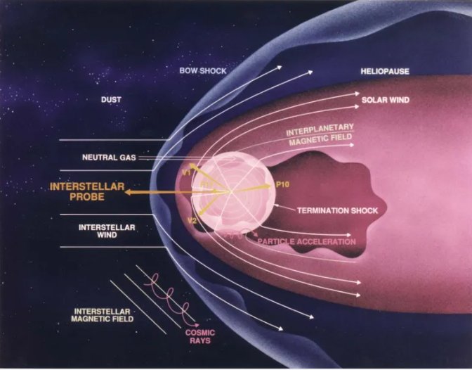
Beyond the termination shock lies the heliosheath — hot, subsonic solar wind plasma. The heliopause is the contact surface separating solar and interstellar plasma. Voyager 1 crossed it at 121 AU in 2012.

If the ISM flow (v_ISM ≈ 26 km/s) is supersonic relative to the ISM sound speed, a bow shock forms upstream. Recent IBEX data suggest the ISM flow is actually sub-fast-magnetosonic, so the bow shock may not exist — replaced by a gradual "bow wave."

1.4.3 Heliospheric Current Sheet

The Sun's magnetic dipole is tilted ≈ 7° from the rotation axis. The equatorial current sheet where B_r reverses sign is warped into a ballerina skirt pattern by solar rotation. Its shape is described by:

$$\theta_{HCS}(\phi, r) = \frac{\pi}{2} + \alpha\sin\!\left(\phi - \frac{\Omega r}{v_r}\right)$$

where α is the tilt angle. This creates sector structure: alternating toward/away magnetic polarity as the sheet sweeps past Earth with the 27-day rotation period.

1.5 Energy Budget of the Solar Wind

The total energy flux in the solar wind at distance r is:

$$F_E = \frac{1}{2}\rho v^2 v_r + \frac{\gamma}{\gamma-1}p v_r - \frac{\rho G M_\odot v_r}{r} + \frac{(\mathbf{E}\times\mathbf{B})_r}{\mu_0}$$

The four terms represent kinetic energy flux, enthalpy flux, gravitational potential energy flux, and Poynting flux (electromagnetic energy). The Poynting flux is:

$$S_r = -\frac{B_\phi v_r B_r - B_r v_\phi B_r}{\mu_0} = -\frac{v_r B_\phi B_r}{\mu_0}$$

At 1 AU, the kinetic energy flux dominates (∼ 99%), and the total solar wind luminosity is:

$$L_{sw} = \frac{1}{2}\dot{M} v^2 \approx \frac{1}{2}(10^9)(4\times10^5)^2 \approx 8\times10^{19} \text{ W} \approx 2\times10^{-7} L_\odot$$

The Coronal Heating Problem

The solar photosphere has T ≈ 5800 K, but the corona is T ≈ 10⁶ K. The mechanism heating the corona to millions of degrees remains one of the great unsolved problems in astrophysics. Leading candidates include:

• Wave heating: Alfvén waves dissipate via phase mixing or turbulent cascade
• Nanoflares: Many small reconnection events (Parker 1988)
• Magnetic braiding: Photospheric motions tangle field lines, driving currents

The required heating rate is ∼10⁵ W/m² for active regions and ∼300 W/m² for quiet Sun.

← Part VII Overview Next: Earth's Magnetosphere →

Plasma Physics Course