Stellar Plasmas
Stars are self-gravitating plasma spheres governed by the equations of stellar structure. This chapter covers the solar corona and its million-degree puzzle, stellar structure equations, mass loss through stellar winds, and magnetohydrostatic equilibria that store energy before explosive release.
4.1 The Solar Corona
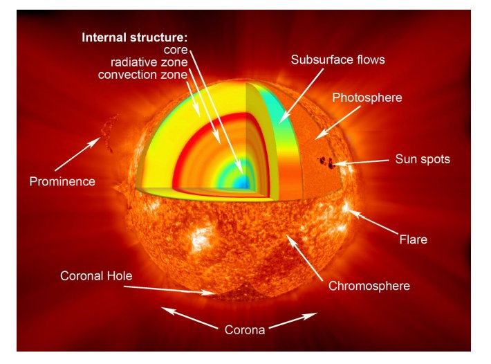
Solar structure — energy flows from the fusion core through radiative and convective zones to the magnetically dominated corona.
The solar corona has T ≈ 1–3 MK, far exceeding the photospheric temperature (~5800 K). Understanding why the corona is so hot is one of the central problems in solar physics.
Derivation: Hydrostatic Scale Height
Step 1. In hydrostatic equilibrium along a radial magnetic field:
Step 2. Using the ideal gas law p = nkBT for an isothermal corona:
Step 3. The solution is exponential with pressure scale height:
For T = 1.5 MK: H ≈ 75 Mm ≈ 0.1 R⊙. This explains why the corona is geometrically extended — the hot plasma has a large scale height.
Derivation: Conductive Temperature Profile
Step 1. Spitzer thermal conductivity parallel to B is dominated by electrons:
Step 2. In a static, radiatively negligible corona, the energy equation reduces to:
Step 3. In spherical symmetry: d/dr(r²κ₀T5/2 dT/dr) = 0, so r²T5/2 dT/dr = const. Integrating:
This very gradual decline (T ∝ r−2/7) explains why the corona remains hot out to several solar radii. The conductive heat flux at the base is:
4.2 The Coronal Heating Problem
The corona loses energy through radiation, conduction to the transition region, and the solar wind. The energy balance for a coronal loop of length L and cross-section A is:
Energy Loss Estimates
Radiative loss: The optically thin radiative loss function Λ(T) peaks near T ~ 105 K (transition region lines) and has a broad minimum near coronal temperatures:
Required heating rates:
- Active regions: ~104 W/m² (at the coronal base)
- Quiet Sun corona: ~300 W/m²
- Coronal holes: ~100 W/m² (mostly conducted back or carried away by wind)
Alfvén Wave Heating
Alfvén waves propagating from the photosphere carry an energy flux:
For photospheric values (δv ~ 1 km/s, B ~ 100 G, ρ ~ 10−4 kg/m³): Fwave ~ 107 W/m² — more than sufficient, but the wave must be damped efficiently. In the corona, phase mixing provides dissipation on a length scale:
Nanoflare Heating (Parker Model)
Parker (1988) proposed that photospheric shuffling of magnetic footpoints braids coronal field lines, building up current sheets that dissipate via reconnection in many small "nanoflares" (E ~ 1024 erg each). The energy input rate is:
where vph ~ 1 km/s is the photospheric shuffling velocity and L is the loop length. This gives a heating rate ~103 W/m², consistent with quiet Sun requirements. The statistical signature would be a power-law distribution of flare energies dN/dE ∝ E−α with α > 2, so that nanoflares dominate the total energy budget.
RTV Scaling Law
For a static coronal loop in radiative and conductive equilibrium, Rosner, Tucker & Vaiana (1978) derived the scaling:
where Tmax is in K, p is pressure in dyn/cm², and L is the half-length in cm. For an active region loop (L ~ 50 Mm, n ~ 1015 m−3, T ~ 3 MK), this successfully predicts the observed scaling between loop length and temperature.
4.3 Stellar Structure Equations
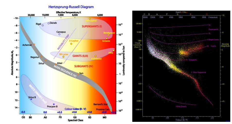
The Hertzsprung-Russell diagram — stellar structure equations predict the main sequence and evolutionary tracks across this diagram.
The interior of a star in thermal equilibrium is described by four coupled ODEs:
Mass conservation:
$$\frac{dm}{dr} = 4\pi r^2 \rho$$Hydrostatic equilibrium:
$$\frac{dp}{dr} = -\frac{Gm(r)\rho}{r^2}$$Luminosity (energy generation):
$$\frac{dL}{dr} = 4\pi r^2 \rho \epsilon(T, \rho)$$Temperature gradient (radiative transport):
$$\frac{dT}{dr} = -\frac{3\kappa \rho L}{64\pi r^2 \sigma_{SB} T^3}$$Derivation: Radiative Temperature Gradient
Step 1. The radiative diffusion equation relates the energy flux to the temperature gradient. In an optically thick medium, photons random-walk with mean free path lmfp = 1/(κρ):
where u = aT⁴ is the radiation energy density (a = 4σSB/c).
Step 2. Differentiating u with respect to r:
Step 3. Setting F = L/(4πr²) and solving for dT/dr:
Derivation: Central Temperature (Virial Theorem)
Step 1. The virial theorem for a self-gravitating gas states:
where U is the thermal energy and Ω is the gravitational potential energy.
Step 2. For a uniform-density sphere: Ω = −3GM²/(5R). The average temperature is related to U by U = (3/2)NkBT̄ = (3/2)(M/mp)kBT̄:
Step 3. Solving for the mean temperature and using Tc ≈ 2T̄ (density weighting):
for solar values. This is close to the actual central temperature of the Sun (1.57 × 10⁷ K), confirming the virial estimate.
4.4 Stellar Winds & Mass Loss
All stars lose mass through winds. The mechanism depends on the stellar type:
- Cool stars (solar-type): Thermally-driven Parker wind (see Ch. 1)
- Hot stars (O, B): Radiation-driven (line-driven) CAK wind
- Red giants: Dust-driven + pulsation-enhanced winds
- Wolf-Rayet: Extremely dense, optically thick radiation-driven winds
Reimers Mass-Loss Formula
For cool giant stars, Reimers (1975) proposed an empirical scaling:
where L, R, M are in solar units and ηR ~ 0.5 is an efficiency parameter. This gives Ṁ ~ 10−14 M⊙/yr for the present Sun, increasing to ~10−8 M⊙/yr on the red giant branch.
Derivation: CAK Radiation-Driven Wind
Step 1. Hot star winds are accelerated by absorption of photospheric UV photons in spectral lines. The line radiation force per unit mass is:
where σe is the electron scattering opacity and M(t) is the force multiplier — a dimensionless factor representing the enhancement due to line absorption. Castor, Abbott & Klein (CAK, 1975) parameterized it as:
where t is the Sobolev optical depth parameter, k ~ 0.1–0.4 and α ~ 0.5–0.7.
Step 2. The equation of motion becomes:
where Γe = σeL/(4πGMc) is the Eddington parameter for electron scattering.
Step 3. The CAK critical solution gives the mass-loss rate:
and the terminal velocity:
For an O5 V star: Ṁ ~ 10−6 M⊙/yr, v∞ ~ 2500 km/s.
Wind Momentum–Luminosity Relation
The modified wind momentum Ṁv∞√R is observed to correlate tightly with luminosity:
with x ≈ 1/α ≈ 1.8 and D depends on spectral type. This provides a powerful extragalactic distance indicator.
4.5 Magnetohydrostatic Equilibria
In the low-β solar corona, magnetic forces dominate gas pressure. The force balance is:
When gas pressure and gravity are negligible, this reduces to the force-free condition:
Force-Free Field Classifications
Potential (α = 0): ∇ × B = 0, so B = −∇Ψ with ∇²Ψ = 0. Minimum-energy state for given boundary flux distribution.
Linear force-free (α = const): ∇²B + α²B = 0 (Helmholtz equation). The constant-α field has minimum energy for given helicity.
Nonlinear force-free (α = α(r)): Most general. B · ∇α = 0 implies α is constant along each field line. Must be solved numerically.
Derivation: Flux Tube Pressure Balance
Consider a magnetic flux tube of radius a embedded in an external pressure pe. Radial pressure balance:
For a straight tube (Bφ = 0), integrating across the boundary:
A flux tube with stronger internal field must have lower internal gas pressure — the basis for sunspot darkening (Wilson depression).
CME: Loss of Equilibrium & Torus Instability
Coronal mass ejections (CMEs) can be understood as a loss of MHD equilibrium. A current-carrying flux rope (modeled as a torus of major radius R and minor radius a) experiences an outward "hoop force":
and is confined by the strapping external field Bex(R). The torus instability occurs when the external field decreases faster than a critical rate:
This decay index criterion n ≥ 3/2 successfully predicts CME onset in both simulations and observations. CME speeds range from 200–3000 km/s with kinetic energies of 1023–1025 J.
Interactive Simulations
Stellar Interior: Fusion Reaction Rates
PythonClick Run to execute the Python code
Code will be executed with Python 3 on the server
Stellar Structure: Hydrostatic Equilibrium
FortranClick Run to execute the Fortran code
Code will be compiled with gfortran and executed on the server